Cubic Spline (cspline) Object
Main.ObjectCspline History
Hide minor edits - Show changes to markup
GEKKO Python Example
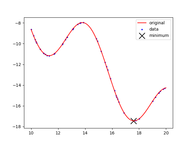
Sample the function `3\sin(x)-(x-3)` at 50 random points between 5 and 15. Use the randomly sampled points to construct a cubic spline and find the minimum of that function.
(:toggle hide gekko button show="Example GEKKO (Python) Code":) (:div id=gekko:)
APM Python Example
Use the following x and y data to construct a cubic spline.
  x_data         ,  y_data
  -1.0000000e+00 ,  3.8461538e-02
  -8.0000000e-01 ,  5.8823529e-02
  -5.0000000e-01 ,  1.3793103e-01
  -2.5000000e-01 ,  3.9024390e-01
   0.0000000e+00 ,  1.0000000e+00
   1.0000000e-01 ,  8.0000000e-01
   2.0000000e-01 ,  5.0000000e-01
   5.0000000e-01 ,  1.3793103e-01
Find the maximum of the interpolated function.
(:toggle hide apm button show="Example APMonitor (Python) Source":) (:div id=apm:)
from gekko import gekko
""" minimize y s.t. y = f(x)
using cubic spline with random sampling of data """
- Function to generate data for cspline
def f(x):
return 3*np.sin(x) - (x-3)
- Create model
c = gekko()
- Cubic spline
x = c.Var(value=15) y = c.Var() x_data = np.random.rand(50)*10+10 y_data = f(x_data) c.cspline(x,y,x_data,y_data,True) c.Obj(y)
- Options
c.options.IMODE = 3 c.options.CSV_READ = 0 c.options.SOLVER = 3 c.solve()
- Generate continuous trend for plot
z = np.linspace(10,20,100)
- Check if solved successfully
if c.options.SOLVESTATUS == 1:
    plt.figure()
    plt.plot(z,f(z),'r-',label='original')
    plt.scatter(x_data,y_data,5,'b',label='data')
    plt.scatter(x.value,y.value,200,'k','x',label='minimum')
    plt.legend(loc='best')
else:
    print ('Failed to converge!')
    plt.figure()
    plt.plot(z,f(z),'r-',label='original')
    plt.scatter(x_data,y_data,5,'b')
    plt.legend(loc='best')
plt.show() (:sourceend:) (:divend:)
APM Python Example
Use the following x and y data to construct a cubic spline.
from APMonitor.apm import *
s = 'https://byu.apmonitor.com' a = 'cspline'
model = ''' Objects
c = cspline
End Objects
File c.csv
Find the maximum of the interpolated function.
(:toggle hide apm button show="Example APMonitor (Python) Source":) (:div id=apm:)
(:source lang=python:) import numpy as np import matplotlib.pyplot as plt from APMonitor.apm import *
s = 'https://byu.apmonitor.com' a = 'cspline'
model = ''' Objects
c = cspline
End Objects
File c.csv
  x_data         ,  y_data
  -1.0000000e+00 ,  3.8461538e-02
  -8.0000000e-01 ,  5.8823529e-02
  -5.0000000e-01 ,  1.3793103e-01
  -2.5000000e-01 ,  3.9024390e-01
   0.0000000e+00 ,  1.0000000e+00
   1.0000000e-01 ,  8.0000000e-01
   2.0000000e-01 ,  5.0000000e-01
   5.0000000e-01 ,  1.3793103e-01
GEKKO Python Example
Sample the function `3\sin(x)-(x-3)` at 50 random points between 5 and 15. Use the randomly sampled points to construct a cubic spline and find the minimum of that function.
(:toggle hide gekko button show="Example GEKKO (Python) Code":) (:div id=gekko:)
(:source lang=python:) from gekko import gekko import numpy as np import matplotlib.pyplot as plt
""" minimize y s.t. y = f(x)
using cubic spline with random sampling of data """
- Function to generate data for cspline
def f(x):
return 3*np.sin(x) - (x-3)
- Create model
c = gekko()
- Cubic spline
x = c.Var(value=15) y = c.Var() x_data = np.random.rand(50)*10+10 y_data = f(x_data) c.cspline(x,y,x_data,y_data,True) c.Obj(y)
- Options
c.options.IMODE = 3 c.options.CSV_READ = 0 c.options.SOLVER = 3 c.solve()
- Generate continuous trend for plot
z = np.linspace(10,20,100)
- Check if solved successfully
if c.options.SOLVESTATUS == 1:
    plt.figure()
    plt.plot(z,f(z),'r-',label='original')
    plt.scatter(x_data,y_data,5,'b',label='data')
    plt.scatter(x.value,y.value,200,'k','x',label='minimum')
    plt.legend(loc='best')
else:
    print ('Failed to converge!')
    plt.figure()
    plt.plot(z,f(z),'r-',label='original')
    plt.scatter(x_data,y_data,5,'b')
    plt.legend(loc='best')
plt.show() (:sourceend:) (:divend:)
See also B-Spline Object for 2D surface function approximations from data
(:toggle hide apm button show="Example APMonitor Model":)
(:toggle hide apm button show="Example APMonitor (Python) Source":)
Sample the function `3\sin(x)-(x-3)` at 50 random points between 5 and 15. Use the randomly sampled points to construct a cubic spline and find the maximum of that function.
Sample the function `3\sin(x)-(x-3)` at 50 random points between 5 and 15. Use the randomly sampled points to construct a cubic spline and find the minimum of that function.
GEKKO Example
GEKKO Python Example
Sample the function `3\sin(x)-(x-3)` at 50 random points between 5 and 15. Use the randomly sampled points to construct a cubic spline and find the maximum of that function.
Sample the function `3\sin(x)-(x-3)` at 50 random points between 5 and 15. Use the randomly sampled points to construct a cubic spline and find the maximum of that function.
APM Python Example
APM Python Example
Use the following x and y data to construct a cubic spline.
  x_data         ,  y_data
  -1.0000000e+00 ,  3.8461538e-02
  -8.0000000e-01 ,  5.8823529e-02
  -5.0000000e-01 ,  1.3793103e-01
  -2.5000000e-01 ,  3.9024390e-01
   0.0000000e+00 ,  1.0000000e+00
   1.0000000e-01 ,  8.0000000e-01
   2.0000000e-01 ,  5.0000000e-01
   5.0000000e-01 ,  1.3793103e-01
Find the maximum of the interpolated function.
Sample the function `3\sin(x)-(x-3)` at 50 random points between 5 and 15. Use the randomly sampled points to construct a cubic spline and find the maximum of that function.
APMonitor Example
APM Python Example
GEKKO Example
APMonitor Example
(:toggle hide gekko button show="Example GEKKO (Python) Code":) (:div id=gekko:)
from gekko import gekko
""" minimize y s.t. y = f(x)
using cubic spline with random sampling of data """
- Function to generate data for cspline
def f(x):
return 3*np.sin(x) - (x-3)
- Create model
c = gekko()
- Cubic spline
x = c.Var(value=15) y = c.Var() x_data = np.random.rand(50)*10+10 y_data = f(x_data) c.cspline(x,y,x_data,y_data,True) c.Obj(y)
- Options
c.options.IMODE = 3 c.options.CSV_READ = 0 c.options.SOLVER = 3 c.solve()
- Generate continuous trend for plot
z = np.linspace(10,20,100)
- Check if solved successfully
if c.options.SOLVESTATUS == 1:
    plt.figure()
    plt.plot(z,f(z),'r-',label='original')
    plt.scatter(x_data,y_data,5,'b',label='data')
    plt.scatter(x.value,y.value,200,'k','x',label='minimum')
    plt.legend(loc='best')
else:
    print ('Failed to converge!')
    plt.figure()
    plt.plot(z,f(z),'r-',label='original')
    plt.scatter(x_data,y_data,5,'b')
    plt.legend(loc='best')
plt.show() (:sourceend:) (:divend:)
(:toggle hide apm button show="Example APMonitor Model":) (:div id=apm:)
(:source lang=python:) import numpy as np import matplotlib.pyplot as plt
(:sourceend:)
(:toggle hide gekko button show="Example GEKKO (Python) Code":) (:div id=gekko:)
(:source lang=python:) from gekko import gekko import numpy as np import matplotlib.pyplot as plt
""" minimize y s.t. y = f(x)
using cubic spline with random sampling of data """
- Function to generate data for cspline
def f(x):
return 3*np.sin(x) - (x-3)
- Create model
c = gekko()
- Cubic spline
x = c.Var(value=15) y = c.Var() x_data = np.random.rand(50)*10+10 y_data = f(x_data) c.cspline(x,y,x_data,y_data,True) c.Obj(y)
- Options
c.options.IMODE = 3 c.options.CSV_READ = 0 c.options.SOLVER = 3 c.solve()
- Generate continuous trend for plot
z = np.linspace(10,20,100)
- Check if solved successfully
if c.options.SOLVESTATUS == 1:
    plt.figure()
    plt.plot(z,f(z),'r-',label='original')
    plt.scatter(x_data,y_data,5,'b',label='data')
    plt.scatter(x.value,y.value,200,'k','x',label='minimum')
    plt.legend(loc='best')
else:
    print ('Failed to converge!')
    plt.figure()
    plt.plot(z,f(z),'r-',label='original')
    plt.scatter(x_data,y_data,5,'b')
    plt.legend(loc='best')
plt.show()
(:toggle hide gekko button show="Example GEKKO (Python) Code":) (:div id=gekko:) (:source lang=python:) from gekko import gekko import numpy as np import matplotlib.pyplot as plt
""" minimize y s.t. y = f(x)
using cubic spline with random sampling of data """
- Function to generate data for cspline
def f(x):
return 3*np.sin(x) - (x-3)
- Create model
c = gekko()
- Cubic spline
x = c.Var(value=15) y = c.Var() x_data = np.random.rand(50)*10+10 y_data = f(x_data) c.cspline(x,y,x_data,y_data,True) c.Obj(y)
- Options
c.options.IMODE = 3 c.options.CSV_READ = 0 c.options.SOLVER = 3 c.solve()
- Generate continuous trend for plot
z = np.linspace(10,20,100)
- Check if solved successfully
if c.options.SOLVESTATUS == 1:
    plt.figure()
    plt.plot(z,f(z),'r-',label='original')
    plt.scatter(x_data,y_data,5,'b',label='data')
    plt.scatter(x.value,y.value,200,'k','x',label='minimum')
    plt.legend(loc='best')
else:
    print ('Failed to converge!')
    plt.figure()
    plt.plot(z,f(z),'r-',label='original')
    plt.scatter(x_data,y_data,5,'b')
    plt.legend(loc='best')
plt.show() (:sourceend:) (:divend:)
(:html:) <iframe width="560" height="315" src="https://www.youtube.com/embed/s1jSLpDXvzs" frameborder="0" allow="autoplay; encrypted-media" allowfullscreen></iframe> (:htmlend:)
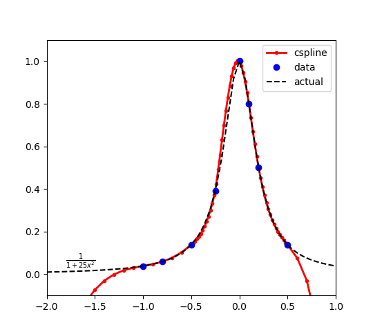
The function is evaluated at the points x_data = [-1.0 -0.8 -0.5 -0.25 0.0 0.1 0.2 0.5].
The function is evaluated at the points x_data = [-1.0 -0.8 -0.5 -0.25 0.0 0.1 0.2 0.5]. Evaluating at additional points shows the cubic spline interpolation function. The maximum of the original function is at x=0 with a result y=1. Because the cubic spline has only 8 points, there is some approximation error and the optimal solution of the cubic spline is slightly to the left of the true solution.
A cubic spline intersects the points to create the function approximations in the range of x between -1.0 and 0.5. There is extrapolation error outside of this range, as expected. Bounds on x should be added or additional cubic spline sample points should be added to avoid problems with optimizer performance in the extrapolation region.
The cubic spline intersects the points to create the function approximations in the range of x between -1.0 and 0.5. There is extrapolation error outside of this range, as expected. Bounds on x should be added or additional cubic spline sample points should be added to avoid problems with optimizer performance in the extrapolation region.
Find the maximum of a function defined by 8 points that approximate the true function.
$$y(x) = \frac{1}{1+25 x^2}$$
The function is evaluated at the points x_data = [-1.0 -0.8 -0.5 -0.25 0.0 0.1 0.2 0.5].
A cubic spline intersects the points to create the function approximations in the range of x between -1.0 and 0.5. There is extrapolation error outside of this range, as expected. Bounds on x should be added or additional cubic spline sample points should be added to avoid problems with optimizer performance in the extrapolation region.
Objects
(:source lang=python:) import numpy as np import matplotlib.pyplot as plt from APMonitor.apm import *
s = 'https://byu.apmonitor.com' a = 'cspline'
model = ''' Objects
 End Objects

 File c.csv
End Objects
File c.csv
 End File

 Connections
End File
Connections
 End Connections

 Variables
End Connections
Parameters End Parameters
Variables
 End Variables

 Equations
End Variables
Equations
End Equations
End Equations '''
- write file
fid = open('model.apm','w') fid.write(model) fid.close()
- clear prior, load new model
apm(s,a,'clear all') apm_load(s,a,'model.apm')
- set steady state optimiation and solve
apm_option(s,a,'apm.imode',3) output = apm(s,a,'solve') print(output)
- retrieve solution
z = apm_sol(s,a)
- print solution
print('x: ' + str(z['x'])) print('y: ' + str(z['y'])) (:sourceend:)
(:title Cubic Spline (cspline) Object:) (:keywords Cubic spline, Object, APMonitor, Option, Configure, Default, Description:) (:description One dimensional cubic spline for nonlinear function approximation with multiple interpolating functions that have continuous first and second derivatives:)

 Type: Object
 Data: Two data vectors that define 1D function points
 Inputs: Name of first data column (e.g. x)
 Outputs: Name of second data column (e.g. y)
 Description: Cubic spline for nonlinear function approximation
A cubic spline is a nonlinear function constructed of multiple third-order polynomials. These polynomials pass through a set of control points and have continuous first and second derivatives everywhere. The second derivative is set to zero at the left and right endpoints, to provide a boundary condition to complete the system of equations. There is poor extrapolation when function retrievals are requested outside of the data points. The input should be constrained or else additional data points added to avoid extrapolation.
Example Usage
 Objects
  c = cspline
 End Objects

 File c.csv
  x_data         ,  y_data
  -1.0000000e+00 ,  3.8461538e-02
  -8.0000000e-01 ,  5.8823529e-02
  -5.0000000e-01 ,  1.3793103e-01
  -2.5000000e-01 ,  3.9024390e-01
   0.0000000e+00 ,  1.0000000e+00
   1.0000000e-01 ,  8.0000000e-01
   2.0000000e-01 ,  5.0000000e-01
   5.0000000e-01 ,  1.3793103e-01
 End File

 Connections
  x = c.x_data
  y = c.y_data
 End Connections

 Variables
  x = -0.5  >= -1 <= 0.5
  y
 End Variables

 Equations
  maximize y
 End Equations