Basis Spline (bspline) Object
Main.ObjectBspline History
Hide minor edits - Show changes to markup
m.Obj(z)
m.Minimize(z)
- raw data
z_data = x*y
xg,yg = np.meshgrid(xgrid,ygrid) z_data = xg*yg
m.Obj(z)
m.Minimize(z)
See also C-Spline Object for 1D function approximations from data
Description: Basis spline for 2D nonlinear approx
Description: Basis spline for 2D nonlinear approximation
Data: Two data vectors and one matrix define the function points
Data: Input (x,y) vectors and output matrix (z)
Description: Basis spline for 2D nonlinear function approximation
Description: Basis spline for 2D nonlinear approx
$$y(x) = \frac{1}{1+25 x^2}$$
The function is evaluated at the points x_data = [-1.0 -0.8 -0.5 -0.25 0.0 0.1 0.2 0.5]. Evaluating at additional points shows the cubic spline interpolation function. The maximum of the original function is at x=0 with a result y=1. Because the cubic spline has only 8 points, there is some approximation error and the optimal solution of the cubic spline is slightly to the left of the true solution.
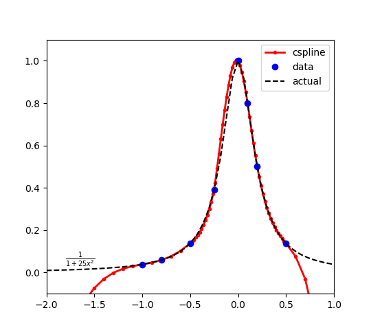
The cubic spline intersects the points to create the function approximations in the range of x between -1.0 and 0.5. There is extrapolation error outside of this range, as expected. Bounds on x should be added or additional cubic spline sample points should be added to avoid problems with optimizer performance in the extrapolation region.
(:title Basis Spline (bspline) Object:) (:keywords Basis spline, b-spline, GEKKO, Object, APMonitor, Option:) (:description Two dimensional basis spline for nonlinear function approximation with multiple interpolating functions that have continuous first and second derivatives:)

 Type: Object
 Data: Two data vectors and one matrix define the function points
 Inputs: b-spline data or knots / coefficients
 Outputs: b-spline appoximation z
 Description: Basis spline for 2D nonlinear function approximation
A basis spline is a nonlinear function constructed of flexible bands that pass through control points to create a smooth curve. The b-spline has continuous first and second derivatives everywhere. The prediction area should be constrained to avoid extrapolation error.
Example Usage
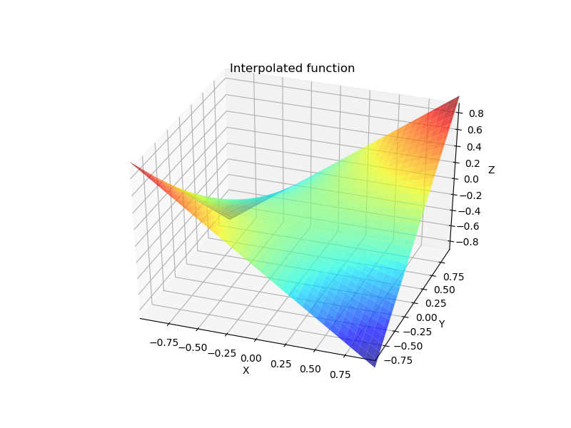
Create a b-spline from the a meshgrid of 50 points in the x-direction and y-direction between -1 and 1 of the function `z=x y`.
(:toggle hide python_bspline button show="Example Python b-spline":) (:div id=python_bspline:) (:source lang=python:) from scipy.interpolate import bisplrep, bisplev import numpy as np import matplotlib.pyplot as plt from mpl_toolkits.mplot3d.axes3d import Axes3D from matplotlib import cm
- Define function over 50x50 grid
xgrid = np.linspace(-1, 1, 50) ygrid = xgrid x, y = np.meshgrid(xgrid, ygrid)
z = x*y
fig = plt.figure(figsize=(8, 6)) ax = fig.add_subplot(111, projection='3d') ax.plot_surface(x,
                y,
                z,
                rstride=2, cstride=2,
                cmap=cm.jet,
                alpha=0.7,
                linewidth=0.25)
plt.title('Sparsely sampled function') ax.set_xlabel('X') ax.set_ylabel('Y') ax.set_zlabel('Z')
- Interpolate function over new 70x70 grid
xgrid2 = np.linspace(-1, 1, 70) ygrid2 = xgrid2 xnew,ynew = np.meshgrid(xgrid2, ygrid2, indexing='ij')
tck = bisplrep(x, y, z, s=0.1) # Build the spline znew = bisplev(xnew[:,0], ynew[0,:], tck) # Evaluate the spline
fig = plt.figure(figsize=(8, 6)) ax = fig.add_subplot(111, projection='3d') ax.plot_surface(xnew,
                ynew,
                znew,
                rstride=2, cstride=2,
                cmap=cm.jet,
                alpha=0.7,
                linewidth=0.25)
plt.title('Interpolated function') ax.set_xlabel('X') ax.set_ylabel('Y') ax.set_zlabel('Z')
plt.show() (:sourceend:) (:divend:)
$$y(x) = \frac{1}{1+25 x^2}$$
The function is evaluated at the points x_data = [-1.0 -0.8 -0.5 -0.25 0.0 0.1 0.2 0.5]. Evaluating at additional points shows the cubic spline interpolation function. The maximum of the original function is at x=0 with a result y=1. Because the cubic spline has only 8 points, there is some approximation error and the optimal solution of the cubic spline is slightly to the left of the true solution.
The cubic spline intersects the points to create the function approximations in the range of x between -1.0 and 0.5. There is extrapolation error outside of this range, as expected. Bounds on x should be added or additional cubic spline sample points should be added to avoid problems with optimizer performance in the extrapolation region.
When creating a bspline object, there are two ways to define the bspline. The first is to define the knots and coefficients directly. Three variables are created as part of the object including:
- object_name.x
- object_name.y
- object_name.z
The x and y are the independent parameters and the z is the dependent variable that is the result of the b-spline evaluation.
(:toggle hide gekko_knots button show="Example Python GEKKO (knots)":) (:div id=gekko_knots:) (:source lang=python:) from gekko import GEKKO import numpy as np
- knots and coeffs
m = GEKKO(remote=False)
tx = [ -1, -1, -1, -1, 1, 1, 1, 1] ty = [ -1, -1, -1, -1, 1, 1, 1, 1] c = [1.0, 0.33333333, -0.33333333, -1.0, 0.33333333, 0.11111111, -0.11111111,
 -0.33333333, -0.33333333, -0.11111111, 0.11111111, 0.33333333, -1.0, -0.33333333,
 0.33333333, 1.0]
x = m.Var(0.5,-1,1) y = m.Var(0.5,-1,1) z = m.Var(2)
m.bspline(x,y,z,tx,ty,c,data=False)
m.Obj(z)
m.solve() (:sourceend:) (:divend:)
(:toggle hide apm_knots button show="Example APMonitor Model (knots)":) (:div id=apm_knots:)
Three files are required including for an APMonitor implementation including:
- object_name_tx.csv (x direction knots)
- object_name_ty.csv (y direction knots)
- object_name_c.csv (b-spline coefficients)
The knots and coefficients can be generated from packages such as Python or MATLAB.
(:source lang=python:)
x direction knots
File b_tx.csv
 -1
 -1
 -1
 -1
  1
  1
  1
  1
End File
y direction knots
File b_ty.csv
 -1
 -1
 -1
 -1
  1
  1
  1
  1
End File
b-spline coefficients
File b_c.csv
 1.0
 0.33333333
 -0.33333333
 -1.0
 0.33333333
 0.11111111
 -0.11111111
 -0.33333333
 -0.33333333
 -0.11111111
 0.11111111
 0.33333333
 -1.0
 -0.33333333
 0.33333333
 1.0
End File
Objects
b = bspline
End Objects
Connections
  x = b.x
  y = b.y
  z = b.z
Parameters
  x = 0.5 > -1 < 1
  y = -0.5 > -1 < 1
Variables
z = 2.0
Equations
minimize z
(:sourceend:) (:divend:)
The second method is to feed in the raw data and let APMonitor or GEKKO generate the knots and coefficients.
(:toggle hide gekko_raw button show="Example Python GEKKO (raw data)":) (:div id=gekko_raw:)
(:source lang=python:) from gekko import GEKKO import numpy as np
- raw data
m = GEKKO(remote=False)
xgrid = np.linspace(-1, 1, 20) ygrid = xgrid z_data = x*y
x = m.Var(0.5,-1,1) y = m.Var(0.5,-1,1) z = m.Var(2)
m.bspline(x,y,z,xgrid,ygrid,z_data)
m.Obj(z)
m.solve() (:sourceend:) (:divend:)
(:toggle hide apm_raw button show="Example APMonitor Model (raw data)":) (:div id=apm_raw:)
Three files are required for the APMonitor implementation including:
- object_name_x.csv (x direction mesh points as 1D vector)
- object_name_y.csv (y direction mesh points as 1D vector)
- object_name_z.csv (z direction mesh grid evaluations as 2D matrix)
(:source lang=python:)
x direction points
File b_x.csv -1.000000000000000000e+00 -9.591836734693877098e-01 -9.183673469387755306e-01 -8.775510204081632404e-01 -8.367346938775510612e-01 -7.959183673469387710e-01 -7.551020408163264808e-01 -7.142857142857143016e-01 -6.734693877551021224e-01 -6.326530612244898322e-01 -5.918367346938775420e-01 -5.510204081632653628e-01 -5.102040816326530726e-01 -4.693877551020408934e-01 -4.285714285714286031e-01 -3.877551020408164240e-01 -3.469387755102041337e-01 -3.061224489795918435e-01 -2.653061224489796643e-01 -2.244897959183673741e-01 -1.836734693877551949e-01 -1.428571428571429047e-01 -1.020408163265307255e-01 -6.122448979591843532e-02 -2.040816326530614511e-02 2.040816326530614511e-02 6.122448979591821328e-02 1.020408163265305035e-01 1.428571428571427937e-01 1.836734693877550839e-01 2.244897959183671521e-01 2.653061224489794423e-01 3.061224489795917325e-01 3.469387755102040227e-01 3.877551020408163129e-01 4.285714285714283811e-01 4.693877551020406713e-01 5.102040816326529615e-01 5.510204081632652517e-01 5.918367346938773199e-01 6.326530612244896101e-01 6.734693877551019003e-01 7.142857142857141906e-01 7.551020408163264808e-01 7.959183673469385489e-01 8.367346938775508391e-01 8.775510204081631294e-01 9.183673469387754196e-01 9.591836734693877098e-01 1.000000000000000000e+00 End File
y direction points
File b_y.csv -1.000000000000000000e+00 -9.591836734693877098e-01 -9.183673469387755306e-01 -8.775510204081632404e-01 -8.367346938775510612e-01 -7.959183673469387710e-01 -7.551020408163264808e-01 -7.142857142857143016e-01 -6.734693877551021224e-01 -6.326530612244898322e-01 -5.918367346938775420e-01 -5.510204081632653628e-01 -5.102040816326530726e-01 -4.693877551020408934e-01 -4.285714285714286031e-01 -3.877551020408164240e-01 -3.469387755102041337e-01 -3.061224489795918435e-01 -2.653061224489796643e-01 -2.244897959183673741e-01 -1.836734693877551949e-01 -1.428571428571429047e-01 -1.020408163265307255e-01 -6.122448979591843532e-02 -2.040816326530614511e-02 2.040816326530614511e-02 6.122448979591821328e-02 1.020408163265305035e-01 1.428571428571427937e-01 1.836734693877550839e-01 2.244897959183671521e-01 2.653061224489794423e-01 3.061224489795917325e-01 3.469387755102040227e-01 3.877551020408163129e-01 4.285714285714283811e-01 4.693877551020406713e-01 5.102040816326529615e-01 5.510204081632652517e-01 5.918367346938773199e-01 6.326530612244896101e-01 6.734693877551019003e-01 7.142857142857141906e-01 7.551020408163264808e-01 7.959183673469385489e-01 8.367346938775508391e-01 8.775510204081631294e-01 9.183673469387754196e-01 9.591836734693877098e-01 1.000000000000000000e+00 End File
evaluation of function for x and y meshgrid
File b_z.csv
all the z data as a matrix (really long)
End File
Objects
b = bspline
End Objects
Connections
  x = b.x
  y = b.y
  z = b.z
Parameters
  x = 0.5 > -1 < 1
  y = -0.5 > -1 < 1
Variables
z = 2.0
Equations
minimize z
(:sourceend:) (:divend:)