Time Delay (Dead-Time)
Model predictive controllers rely on dynamic models of the process, most often linear empirical models obtained by system identification. APMonitor and GEKKO support continuous or discrete state space and autoregressive exogenous (ARX) input models. The delay function implements dead-time and is a simplified ARX model that includes a single input and output with a delay structure specified by the number of integer time steps.
  Usage: delay(u,y,steps=1)
    u = delay input
    y = delay output
    steps = integer number of steps (default=1)
  Description: Build a delay with number of time steps between
    input (u) and output (y) with a time series model.
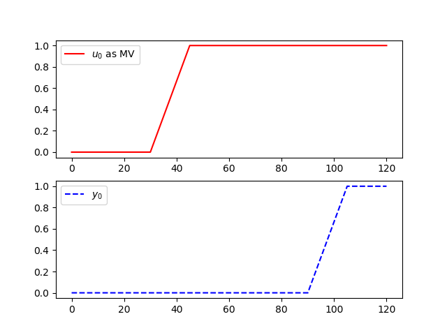
The following is an example of implementing a discrete time series model for an input delay of 60 seconds. The sample time for this model is 15 seconds with 4 steps of delay. The model is implemented in Gekko with the delay function.

from gekko import GEKKO
import matplotlib.pyplot as plt
# Create GEKKO model
m = GEKKO()
cv = m.Var()
mv = m.Param()
m.delay(mv,cv,4)
m.time = np.linspace(0,120,9)
mv.value = np.zeros(9)
mv.value[3:9] = 1
m.options.imode = 4
m.options.nodes = 2
m.solve() # (GUI=True)
# also create a Python plot
import matplotlib.pyplot as plt
plt.subplot(2,1,1)
plt.plot(m.time,mv.value,'r-',label=r'MV')
plt.legend()
plt.subplot(2,1,2)
plt.plot(m.time,cv.value,'b--',label=r'$CV$')
plt.legend()
plt.show()
Also see