APMonitor

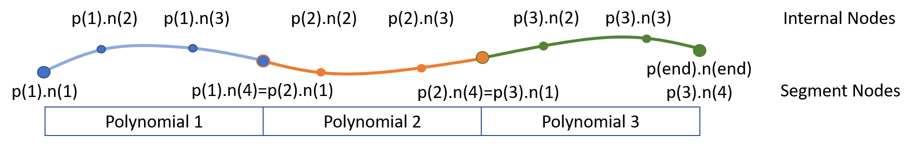
In this example illustration, the number of nodes is 4 and the number of time segments is 3 such as defined by these 4 time points: [0,1,2,3]. Successive endpoints of the time segments are merged to form a chain of model predictions. The `end` designation can be used for the polynomial segments or the nodes with `p(3)=p(end)` and `n(4)=n(end)` for the example above. Increasing the number of nodes will generally improve the solution accuracy but also increase the problem size and computation time. Solution accuracy can also be improved by adding more time segments. APMonitor and APM Matlab use index-1 for the polynomial time positions while Gekko and Python use index-0. The node positions are index-1 for both APMonitor and Gekko. To facilitate common functions to fix or free initial or end points, the following Gekko functions are available.

(:source lang=python:) from gekko import GEKKO m = GEKKO() x = m.Var() m.fix_initial(x) m.fix_final(x) m.free_initial(x) m.free_final(x) (:sourceend:)

A more detailed description of NODES is given in the lecture material on Orthogonal Collocation on Finite Elements with example problems. An additional example problem is shown below.

with initial condition `y_0=5`. Show the internal node solutions.

In this example illustration, the number of nodes is 4 and the number of time segments is 3 such as defined by these 4 time points: [0,1,2,3]. Successive endpoints of the time segments are merged to form a chain of model predictions. Increasing the number of nodes will generally improve the solution accuracy but also increase the problem size and computation time. Solution accuracy can also be improved by adding more time segments. A more detailed description of NODES is given in the lecture material on Orthogonal Collocation on Finite Elements with the associated example problems.

Example Problem

Solve the equation with NODES=4 at time points [0,1,2,3]:

and show the internal node solutions.

Solution

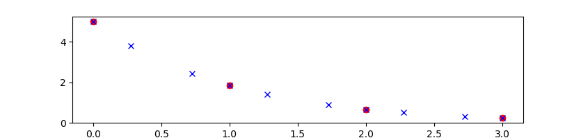
(:source lang=python:) from gekko import GEKKO m = GEKKO(remote=False) # create GEKKO model y = m.Var(5.0,name='y') # create GEKKO variable m.Equation(y.dt()==-y) # create GEKKO equation m.time = [0,1,2,3] # time points m.options.IMODE = 4 # simulation mode m.options.NODES = 4 # set NODES=4 m.options.CSV_WRITE=2 # write results_all.json

                        #   with internal nodes

m.solve() # solve m.open_folder() # open run folder to see

                        #   source and results files

import matplotlib.pyplot as plt

1. plot at [0,1,2,3]

plt.plot(m.time,y,'ro')

1. retrieve internal nodes from results_all.json

import json with open(m.path+'//results_all.json') as f:

    results = json.load(f)

plt.plot(results['time'],results['y'],'bx') plt.show() (:sourceend:)

In this example illustration, the number of nodes is 4 and the number of time segments is 3 such as defined by these 4 time points: [0,1,2,3].

$$\frac{dy}{dt}=-y$$

Successive endpoints of the time segments are merged to form a chain of model predictions. Increasing the number of nodes will generally improve the solution accuracy but also increase the problem size and computation time. Solution accuracy can also be improved by adding more time segments. A more detailed description of NODES is given in the lecture material on Orthogonal Collocation on Finite Elements with the associated example problems.

NODES are the number of collocation points in the span of each time segment. For dynamic problems, the time segments are linked together into a time horizon as shown in the figure below.

In this example illustration, the number of nodes is 4 and the number of time segments is 3 such as defined by these 4 time points: [0,1,2,3]. Successive endpoints of the time segments are merged to form a chain of model predictions. Increasing the number of nodes will generally improve the solution accuracy but also increase the problem size and computation time. Solution accuracy can also be improved by adding more time segments. A more detailed description of NODES is given in the lecture material on Orthogonal Collocation on Finite Elements with the associated example problems.

NODES are the number of collocation points in the span of each time segment. For dynamic problems, the time segments are linked together into a time horizon. Successive endpoints of the time segments are merged to form a chain of model predictions. Increasing the number of nodes will generally improve the solution accuracy but also increase the problem size and computation time. Solution accuracy can also be improved by adding more time segments. A more detailed description of NODES is given in the lecture material on Orthogonal Collocation on Finite Elements with the associated example problems.

 Allowable Range: 2-6

See also CTRL_HOR, CTRL_TIME, CTRL_UNITS, HIST_UNITS, PRED_HOR, PRED_TIME

(:title APM.NODES - APMonitor Option:) (:keywords APM.NODES, Optimization, Estimation, Option, Configure, Default, Description:) (:description Nodes in each horizon step:)

 Type: Integer, Input
 Default Value: 3
 Description: Nodes in each horizon step

NODES are the number of collocation points in the span of each time segment. For dynamic problems, the time segments are linked together into a time horizon. Successive endpoints of the time segments are merged to form a chain of model predictions. Increasing the number of nodes will generally improve the solution accuracy but also increase the problem size and computation time. Solution accuracy can also be improved by adding more time segments.