See also: Optimal measles vaccine distribution

Solution (Python GEKKO)

(:toggle hide gekko button show="Show GEKKO (Python) Code":) (:div id=gekko:) Thanks to Cameron Price for providing the GEKKO Python code.

Estimate 26 beta values and gamma

(:source lang=python:) import numpy as np from gekko import GEKKO import matplotlib.pyplot as plt

1. Import Data
2. write csv data file

t_s = np.linspace(0,78,79)

1. case data

cases_s = np.array([180,180,271,423,465,523,649,624,556,420, 423,488,441,268,260,163,83,60,41,48,65,82, 145,122,194,237,318,450,671,1387,1617,2058, 3099,3340,2965,1873,1641,1122,884,591,427,282, 174,127,84,97,68,88,79,58,85,75,121,174,209,458, 742,929,1027,1411,1885,2110,1764,2001,2154,1843, 1427,970,726,416,218,160,160,188,224,298,436,482,468])

1. Initialize gekko model

m = GEKKO()

1. Number of collocation nodes

nodes = 4

1. Number of phases (years in this case)

n = 3

1. Biweek periods per year

bi = 26

1. Time horizon (for all 3 phases)

m.time = np.linspace(0,1,bi+1)

1. Parameters that will repeat each year

N = m.Param(3.2e6) mu = m.Param(7.8e-4) rep_frac = m.Param(0.45) Vr = m.Param(0)

beta = m.MV(2,lb = 0.1) beta.STATUS = 1

gamma = m.FV(value=0.07) gamma.STATUS = 1 gamma.LOWER = 0.05 gamma.UPPER = 0.5

1. Data used to control objective function

casesobj1 = m.Param(cases_s[0:(bi+1)]) casesobj2 = m.Param(cases_s[bi:(2*bi+1)]) casesobj3 = m.Param(cases_s[2*bi:(3*bi+1)])

1. Variables that vary between years, one version for each year

cases = [m.CV(value = cases_s[(i*bi):(i+1)*(bi+1)-i],lb=0) for i in range(n)] for i in cases:

    i.FSTATUS = 1
    i.WMODEL = 0
    i.MEAS_GAP = 100

S = [m.Var(0.06*N,lb = 0,ub = N) for i in range(n)] I = [m.Var(0.001*N, lb = 0,ub = N) for i in range(n)] V = [m.Var(2e5) for i in range(n)]

1. Equations (created for each year)

for i in range(n):

    R = m.Intermediate(beta*S[i]*I[i]/N)
    m.Equation(S[i].dt() == -R + mu*N - Vr)
    m.Equation(I[i].dt() == R - gamma*I[i])
    m.Equation(cases[i] == rep_frac*R)
    m.Equation(V[i].dt() == -Vr)

1. Connect years together at endpoints

for i in range(n-1):

    m.Connection(cases[i+1],cases[i],1,bi,1,nodes)#,1,nodes)
    m.Connection(cases[i+1],'CALCULATED',pos1=1,node1=1)
    m.Connection(S[i+1],S[i],1,bi,1,nodes)
    m.Connection(S[i+1],'CALCULATED',pos1=1,node1=1)
    m.Connection(I[i+1],I[i],1,bi,1,nodes)
    m.Connection(I[i+1],'CALCULATED',pos1=1, node1=1)

1. Solver options

m.options.IMODE = 5 m.options.NODES = nodes m.EV_TYPE = 1 m.options.SOLVER = 1

1. Solve

m.Obj(2*(casesobj1-cases[0])**2+(casesobj3-cases[2])**2)

m.solve()

1. Calculate the start time of each phase

ts = np.linspace(1,n,n)

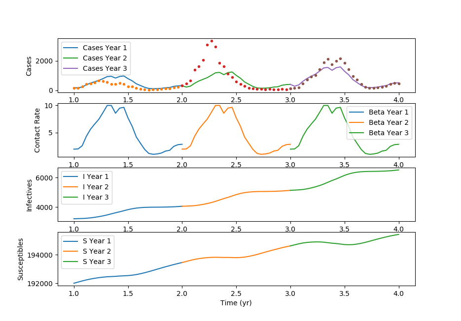
1. Plot

plt.figure() plt.subplot(4,1,1) tm = np.empty(len(m.time)) for i in range(n):

    tm = m.time + ts[i]
    plt.plot(tm,cases[i].value,label='Cases Year (i+1))
    plt.plot(tm,cases_s[(i*bi):(i+1)*(bi+1)-i],'.')

plt.legend() plt.ylabel('Cases')

plt.subplot(4,1,2) for i in range(n):

    tm = m.time + ts[i]
    plt.plot(tm,beta.value,label='Beta Year (i+1))

plt.legend() plt.ylabel('Contact Rate')

plt.subplot(4,1,3) for i in range(n):

    tm = m.time + ts[i]
    plt.plot(tm,I[i].value,label='I Year (i+1))

plt.legend() plt.ylabel('Infectives')

plt.subplot(4,1,4) for i in range(n):

    tm = m.time + ts[i]
    plt.plot(tm,S[i].value,label='S Year (i+1))

plt.legend() plt.ylabel('Susceptibles') plt.xlabel('Time (yr)')

plt.show() (:sourceend:) (:divend:)

Understanding the spread of the measles virus from historical data of major metropolitan areas will help researchers understand the fundamentals of disease spread through a population. This may help guide policy for school closure, travel restrictions, and other measures intended to slow disease spread until a vaccine can be developed or deployed.

References

• Daniel P. Word, George H. Abbott, Derek Cummings, and Carl D. Laird, "Estimating Seasonal Drivers in Childhood Infectious Diseases with Continuous Time and Discrete-Time Models", in Proceedings, 2010 American Control Conference, pp. 5137-5142, Baltimore, MD, June 29 - July 2, 2010.
• Daniel P. Word, James K. Young, Derek Cummings, Carl D. Laird, "Estimation of seasonal transmission parameters in childhood infectious disease using a stochastic continuous time model", Computer Aided Chemical Engineering, pp. 229-234, 28, 2010.

(:source lang=python:)

(:sourceend:)

Daniel P. Word, George H. Abbott, Derek Cummings, and Carl D. Laird, "Estimating Seasonal Drivers in Childhood Infectious Diseases with Continuous Time and Discrete-Time Models", in Proceedings, 2010 American Control Conference, Baltimore, MD, June 29 - July 2, 2010, p. 5137-5142.

Control Measles Outbreak with Optimal Vaccination Scheduling

(:html:) <iframe width="560" height="315" src="https://www.youtube.com/embed/UTTlZ6rVXxM" frameborder="0" allowfullscreen></iframe> (:htmlend:)

Reference

   Daniel P. Word, George H. Abbott, Derek Cummings, and Carl D. Laird, "Estimating Seasonal Drivers in Childhood Infectious Diseases with Continuous Time and Discrete-Time Models", in Proceedings, 2010 American Control Conference, Baltimore, MD, June 29 - July 2, 2010, p. 5137-5142.

(:title Simulation of Infectious Disease Spread:) (:keywords nonlinear, model, predictive control, APMonitor, differential, algebraic, modeling language, infectious disease spread, measles nonlinear dynamics:) (:description Simulation of infectious disease spread (measles) with APMonitor:)

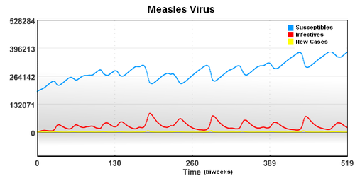
In this case, the starting population of 3,200,000 is composed of a group of Susceptible, Infected, and Recovered individuals. To account for underreporting of measles cases, a reporting factor is used in the model. In this study, it is assumed that only 45% of the measles cases were reported.

Measles (sometimes known as English Measles) is spread through respiration (contact with fluids from an infected person's nose and mouth, either directly or through aerosol transmission), and is highly contagious—90% of people without immunity sharing living space with an infected person will catch it. The infection has an average incubation period of 14 days (range 6–19 days) and infectivity lasts from 2–4 days prior, until 2–5 days following the onset of the rash (i.e. 4–9 days infectivity in total).

Understanding the spread of the measles virus from historical data of major metropolitan areas will help researchers understand the fundamentals of disease spread through a population. This may help guide policy for school closure, travel restrictions, and other measures intended to slow disease spread until a suitable vaccine can be developed.

In this case, the starting population of 3,200,000 is composed of a group of Susceptible, Infectived, and Recovered individuals. To account for underreporting of measles cases, a reporting factor is used in the model. In this study, it is assumed that only 45% of the measles cases were reported.

The seasonal transmission parameter can also be used to estimate spread of other diseases. The transmission parameter is the number of contact (on average) made with other individuals during a biweek period. The transmission parameter can sometimes be decreased for brief periods of time to slow the spread of a disease. Also, the number of susceptible individuals can be reduced through the use of vaccines. In the case of limited vaccine supply, disease spread models can help identify the best use the resources to limit large outbreaks.

Measles (sometimes known as English Measles) is spread through respiration (contact with fluids from an infected person's nose and mouth, either directly or through aerosol transmission), and is highly contagious—90% of people without immunity sharing living space with an infected person will catch it. The infection has an average incubation period of 14 days (range 6–19 days) and infectivity lasts from 2–4 days prior, until 2–5 days following the onset of the rash (i.e. 4–9 days infectivity in total). Understanding the spread of the measles virus from historical data of major metropolitan areas will help researchers understand the spread of disease through a population. In this case, the starting population of 3,200,000 is composed of a group of Susceptible, Infectived, and Recovered individuals.

To account for underreporting of measles cases, a reporting factor is used in the model. In this case, it is assumed that only 45% of the measles cases were reported as new cases.

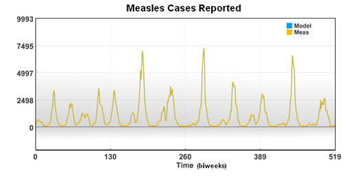
The new case data shows a seasonal variation that is caused by an increased rate of contact between the susceptible population and the infective population. Based on the new case data (cases), birth rate (mu), and recovery rate (gamma), the seasonal variation of the transmission parameter is estimated over a period of 20 years.

The seasonal transmission parameter can be used to estimate spread of other diseases. The transmission parameter is the number of contact (on average) made with other individuals during a biweek period.

    ! birth rate             (births/biweek/total population)

Measles Virus Spread

(:html:)<font size=2><pre>

APMonitor Modeling Language

Data from New York for the years 1947-1965

Data from Bangkok for the years 1975-1984

Data from London is 1944-1966?

Model disease

  Parameters
    ! population size        (individuals)
    N           = 3.2e6               
     ! birth rate             (births/biweek/total population)
    mu          = 7.8e-4             
    ! recovery rate          (recoveries/biweek/infectives)
    gamma       = 0.07              
    ! reporting fraction to account for underreporting                
    rep_frac    = 0.45
    ! cases reported         (new individuals infected per biweek)
    cases = 180, >= 0                 
  End Parameters

  Variables
    ! transmission parameter (potentially infectious contacts/biweek)
    beta = 10
    ! susceptibles           (individuals in the total population)
    S = 0.06*N, >= 0, <= N
    ! infectives             (individuals infected)
    I = 0.0001*N, >= 0, <= N
  End Variables

  Intermediates
    ! infection rate per biweek
    R = beta * S * I / N
  End Intermediates

  Equations
    $S = -R +  mu * N
    $I =  R -  gamma * I
    cases = rep_frac * R
  End Equations

End Model </pre></font>(:htmlend:)

References

Daniel P. Word, George H. Abbott, Derek Cummings, and Carl D. Laird, "Estimating Seasonal Drivers in Childhood Infectious Diseases with Continuous Time and Discrete-Time Models", in Proceedings, 2010 American Control Conference, Baltimore, MD, June 29 - July 2, 2010, p. 5137-5142.