Brachistochrone Optimal Control
Apps.BrachistochroneProblem History
Show minor edits - Show changes to markup
(:html:)
 <div id="disqus_thread"></div>
    <script type="text/javascript">
        /* * * CONFIGURATION VARIABLES: EDIT BEFORE PASTING INTO YOUR WEBPAGE * * */
        var disqus_shortname = 'apmonitor'; // required: replace example with your forum shortname

        /* * * DON'T EDIT BELOW THIS LINE * * */
        (function() {
            var dsq = document.createElement('script'); dsq.type = 'text/javascript'; dsq.async = true;
            dsq.src = 'https://' + disqus_shortname + '.disqus.com/embed.js';
            (document.getElementsByTagName('head')[0] || document.getElementsByTagName('body')[0]).appendChild(dsq);
        })();
    </script>
    <noscript>Please enable JavaScript to view the <a href="https://disqus.com/?ref_noscript">comments powered by Disqus.</a></noscript>
    <a href="https://disqus.com" class="dsq-brlink">comments powered by <span class="logo-disqus">Disqus</span></a>
(:htmlend:)
$$\quad \frac{dx(t)}{dt} = v sin(u)$$
$$\quad \frac{dy(t)}{dt} = v cos(u)$$
$$\quad \frac{dv(t)}{dt} = g cos(u)$$
$$\quad \frac{dx(t)}{dt} = v \; \sin(u)$$
$$\quad \frac{dy(t)}{dt} = v \; \cos(u)$$
$$\quad \frac{dv(t)}{dt} = g \; \cos(u)$$
$$\mathrm{subject/;to}$$
$$\mathrm{subject\;to}$$
$$\mathrm{subject to}$$
$$\mathrm{subject/;to}$$
$$subject to$$
$$\mathrm{subject to}$$
$$"subject to"$$
$$subject to$$
$$\quad x(t_f)=2, \quad y(t_f)=2, \quad v(t_f)="Free"$$
$$\quad x(t_f)=2, \quad y(t_f)=2, \quad v(t_f)=Free$$
(:html:) <iframe width="560" height="315" src="https://www.youtube.com/embed/pgJ0jbfFBUE" frameborder="0" allowfullscreen></iframe> (:htmlend:)

The adjustable parameter u is the slope and can be adjusted over the minimized time horizon tf. The variable x is the horizontal position and y is the vertical position while v is the velocity. The parameter g is the gravitational constant (assume 9.81 m/s2).
The adjustable parameter u is the slope and can be adjusted over the minimized time horizon tf. The variable x is the horizontal position and y is the vertical position in the down direction while v is the velocity. The parameter g is the gravitational constant (assume 9.81 m/s2).
Thanks to Trent Okeson for providing a solution to this problem.
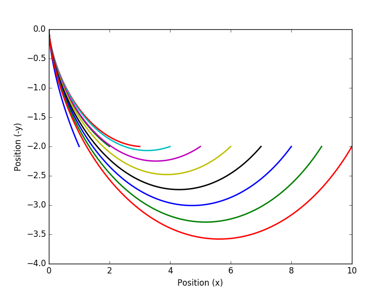
An interesting extension to this problem is to compare the solutions to when the value of x is varied from 1.0 to 10.0. The final value of y is fixed at 2.0 below the starting point.
Thanks to Trent Okeson for providing a solution to this problem.
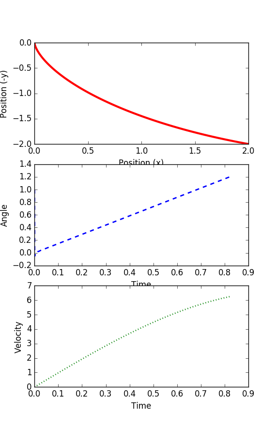
Solution
Thanks to Trent Okeson for providing a solution to this problem.
This is a classic problem that has been solved with calculus of variations but this particular task is to use a numerical method to solve this same problem. The solution curve is independent of both gravitational force and the mass of the object. The solution is different if there is an initial velocity or if there is friction. The adjustable parameter u is the slope and can be adjusted over the minimized time horizon tf. The variable x is the horizontal position and y is the vertical position while v is the velocity. The parameter g is the gravitational constant (assume 9.81 m/s2).
This is a classic problem that has been solved with calculus of variations but this particular task is to use a numerical method to solve this same problem. The solution curve is independent of both gravitational force and the mass of the object. The solution is different if there is an initial velocity or if there is friction.
The adjustable parameter u is the slope and can be adjusted over the minimized time horizon tf. The variable x is the horizontal position and y is the vertical position while v is the velocity. The parameter g is the gravitational constant (assume 9.81 m/s2).
$$\quad x(0)=0, y(0)=0, v(0)=0$$
$$\quad x(t_f)=2, y(t_f)=2, v(t_f)="Free"$$
$$\quad x(0)=0, \quad y(0)=0, \quad v(0)=0$$
$$\quad x(t_f)=2, \quad y(t_f)=2, \quad v(t_f)="Free"$$
$$\quad x(t_f)=2, y(t_f)=2, v(t_f)=Free$$
$$\quad x(t_f)=2, y(t_f)=2, v(t_f)="Free"$$
$$\mathrm{subject to}$$
$$\mathtt subject to$$
$$subject to$$
$$\tt{subject to}$$
$$ x(0)=0, y(0)=0, v(0)=0$$
$$ x(t_f)=2, y(t_f)=2, v(t_f)=Free$$
$$\quad x(0)=0, y(0)=0, v(0)=0$$
$$\quad x(t_f)=2, y(t_f)=2, v(t_f)=Free$$
 minimize tf

 subject to
    dx/dt = v * sin(u)
    dy/dt = v * cos(u)
    dv/dt = g * cos(u)

 initial boundary conditions
    x(0) = 0
    x(0) = 0
    v(0) = 0

 final boundary conditions
    x(tf) = 2
    y(tf) = 2
    v(tf) = Free
$$\min t_f$$
$$subject to$$
$$\quad \frac{dx(t)}{dt} = v sin(u)$$
$$\quad \frac{dy(t)}{dt} = v cos(u)$$
$$\quad \frac{dv(t)}{dt} = g cos(u)$$
$$ x(0)=0, y(0)=0, v(0)=0$$
$$ x(t_f)=2, y(t_f)=2, v(t_f)=Free$$
This is a classic problem that has been solved with calculus of variations but this particular task is to use a numerical method to solve this same problem. The solution curve is independent of both gravitational force and the mass of the object. The solution is different if there is an initial velocity or if there is friction. The adjustable parameter u is the slope and can be adjusted over the minimized time horizon tf. The variable x is the horizontal position and y is the vertical position. The parameter g is the gravitational constant (assume 9.81 m/s2).
This is a classic problem that has been solved with calculus of variations but this particular task is to use a numerical method to solve this same problem. The solution curve is independent of both gravitational force and the mass of the object. The solution is different if there is an initial velocity or if there is friction. The adjustable parameter u is the slope and can be adjusted over the minimized time horizon tf. The variable x is the horizontal position and y is the vertical position while v is the velocity. The parameter g is the gravitational constant (assume 9.81 m/s2).
This is a classic problem that has been solved with calculus of variations but this particular task is to use a numerical method to solve this same problem. The solution curve is independent of both gravitational force and the mass of the object. The solution is different if there is an initial velocity or if there is friction. The adjustable parameter u is the slope and can be adjusted over the minimized time horizon tf. The variable x is the horizontal position and y is the vertical position. The parameter g is the gravitational constant (assume 9.81 m/s2).
This is a classic problem that has been solved with calculus of variations but this particular task is to use a numerical method to solve this same problem. The solution curve is independent of both gravitational force and the mass of the object. The solution is different if there is an initial velocity or if there is friction. The adjustable parameter u is the slope and can be adjusted over the minimized time horizon tf. The variable x is the horizontal position and y is the vertical position. The parameter g is the gravitational constant (assume 9.81 m/s2).
This is a classic problem that has been solved with calculus of variations but this particular task is to use a numerical method to solve this same problem. The solution curve is independent of both gravitational force and the mass of the object. The solution is different if there is an initial velocity or if there is friction. The adjustable parameter u is the slope and can be adjusted over the minimized time horizon tf. The variable x is the horizontal position and y is the vertical position. The parameter g is the gravitational constant (assume 9.81 m/s^2).
This is a classic problem that has been solved with calculus of variations but this particular task is to use a numerical method to solve this same problem. The solution curve is independent of both gravitational force and the mass of the object. The solution is different if there is an initial velocity or if there is friction. The adjustable parameter u is the slope and can be adjusted over the minimized time horizon tf. The variable x is the horizontal position and y is the vertical position. The parameter g is the gravitational constant (assume 9.81 m/s2).
This is a classic problem that has been solved with calculus of variations. This particular demonstration is a numerical method to solve this same problem. The solution curve is independent of both gravitational force and the mass of the object. The solution is different if there is an initial velocity or if there is friction.
This is a classic problem that has been solved with calculus of variations but this particular task is to use a numerical method to solve this same problem. The solution curve is independent of both gravitational force and the mass of the object. The solution is different if there is an initial velocity or if there is friction. The adjustable parameter u is the slope and can be adjusted over the minimized time horizon tf. The variable x is the horizontal position and y is the vertical position. The parameter g is the gravitational constant (assume 9.81 m/s^2).
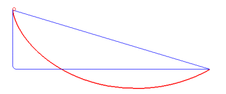
A classic optimal control problem is to compute the brachistochrone curve of fastest descent. A point mass must slide without friction and with constant gravitational force to an fixed end point in the shortest time.
A classic optimal control problem is to compute the brachistochrone curve of fastest descent. A point mass must slide without friction and with constant gravitational force to an fixed end point in the shortest time. The following animation (source: Wikipedia) shows different trial solutions (blue) and the optimal solution (red) for a particular starting and end point.
A classic optimal control problem is to compute the brachistochrone curve of fastest descent. A point mass must slide without friction and with constant gravitational force to an fixed end point in the shortest time. This is a classic problem that has been solved with calculus of variations. This particular demonstration is a numerical method to solve this same problem. The solution curve is independent of both gravitational force and the mass of the object. The solution is different if there is an initial velocity or if there is friction.
A classic optimal control problem is to compute the brachistochrone curve of fastest descent. A point mass must slide without friction and with constant gravitational force to an fixed end point in the shortest time.
This is a classic problem that has been solved with calculus of variations. This particular demonstration is a numerical method to solve this same problem. The solution curve is independent of both gravitational force and the mass of the object. The solution is different if there is an initial velocity or if there is friction.
A classic optimal control problem is to compute the brachistochrone curve of fastest descent. A point mass must slide without friction and with constant gravitational force to an fixed end point in the shortest time. This is a classic problem that has been solved with calculus of variations. This particular demonstration is a numerical method to solve this same problem. The solution curve is independent of both gravitational force and the mass of the object. The solution is different if there is an initial velocity or if there is friction.
A classic optimal control problem is to compute the brachistochrone curve of fastest descent. A point mass must slide without friction and with constant gravitational force to an fixed end point in the shortest time. This is a classic problem that has been solved with calculus of variations. This particular demonstration is a numerical method to solve this same problem. The solution curve is independent of both gravitational force and the mass of the object. The solution is different if there is an initial velocity or if there is friction.
(:title Brachistochrone Solution with MATLAB and Python:)
(:title Brachistochrone Optimal Control:)
A classic optimal control problem is to compute the brachistochrone curve of fastest descent. A point mass must slide without friction and with constant gravitational force to an fixed end point in the shortest time. The problem has been solved with calculus of variations. This is a demonstration of a numerical method to solve this same problem. The solution curve is independent of both gravitational force and the mass of the object. The solution is different if there is an initial velocity or if there is friction.
A classic optimal control problem is to compute the brachistochrone curve of fastest descent. A point mass must slide without friction and with constant gravitational force to an fixed end point in the shortest time. This is a classic problem that has been solved with calculus of variations. This particular demonstration is a numerical method to solve this same problem. The solution curve is independent of both gravitational force and the mass of the object. The solution is different if there is an initial velocity or if there is friction.
(:title Brachistochrone Solution with MATLAB and Python:) (:keywords Python, MATLAB, nonlinear control, Brachistochrone, dynamic programming, optimal control:) (:description Minimize final time on which a bead slides without friction under the influence of a uniform gravitational field to a given end point in the shortest time.:)
A classic optimal control problem is to compute the brachistochrone curve of fastest descent. A point mass must slide without friction and with constant gravitational force to an fixed end point in the shortest time. The problem has been solved with calculus of variations. This is a demonstration of a numerical method to solve this same problem. The solution curve is independent of both gravitational force and the mass of the object. The solution is different if there is an initial velocity or if there is friction.
Problem Statement
 minimize tf

 subject to
    dx/dt = v * sin(u)
    dy/dt = v * cos(u)
    dv/dt = g * cos(u)

 initial boundary conditions
    x(0) = 0
    x(0) = 0
    v(0) = 0

 final boundary conditions
    x(tf) = 2
    y(tf) = 2
    v(tf) = Free
Solution
(:html:)
 <div id="disqus_thread"></div>
    <script type="text/javascript">
        /* * * CONFIGURATION VARIABLES: EDIT BEFORE PASTING INTO YOUR WEBPAGE * * */
        var disqus_shortname = 'apmonitor'; // required: replace example with your forum shortname

        /* * * DON'T EDIT BELOW THIS LINE * * */
        (function() {
            var dsq = document.createElement('script'); dsq.type = 'text/javascript'; dsq.async = true;
            dsq.src = 'https://' + disqus_shortname + '.disqus.com/embed.js';
            (document.getElementsByTagName('head')[0] || document.getElementsByTagName('body')[0]).appendChild(dsq);
        })();
    </script>
    <noscript>Please enable JavaScript to view the <a href="https://disqus.com/?ref_noscript">comments powered by Disqus.</a></noscript>
    <a href="https://disqus.com" class="dsq-brlink">comments powered by <span class="logo-disqus">Disqus</span></a>
(:htmlend:)