Electric Car Optimization
Apps.ElectricVehicleEnergy History
Show minor edits - Show changes to markup
Electric car optimization finds the optimal control strategy for driving an electric car 100 meters in 10 seconds while minimizing energy consumption. The mathematical model uses ordinary differential equations (ODEs) to describe the car behavior. The manipulated variable is the voltage input to the motor, which can accelerate or recharge the battery with regenerative braking. The manipulated variable `p(t)` is a dimensionless variable bounded between -1 and 1. It scales the battery voltage `V_{b}` to regulate the electric current `i(t)` in the motor:
Electric car optimization finds the optimal control strategy for driving an electric car 100 meters in 10 seconds while minimizing energy consumption. The mathematical model uses ordinary differential equations (ODEs) to describe the car behavior. The manipulated variable is the voltage input to the motor, which can accelerate or recharge the battery with regenerative braking.
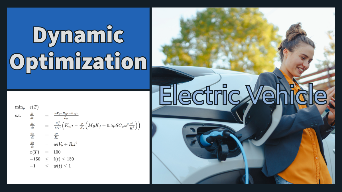
The manipulated variable `p(t)` is a dimensionless variable bounded between -1 and 1. It scales the battery voltage `V_{b}` to regulate the electric current `i(t)` in the motor:
The electric car optimization problem involves finding the optimal control strategy for driving an electric car 100 meters in 10 seconds while minimizing energy consumption. The mathematical model uses ordinary differential equations (ODEs) to describe the car behavior. The manipulated variable is the voltage input to the motor, which can accelerate or recharge the battery with regenerative braking.
The manipulated variable `p(t)` is a dimensionless variable bounded between -1 and 1. It scales the battery voltage `V_{b}` to regulate the electric current `i(t)` in the motor:
Electric car optimization finds the optimal control strategy for driving an electric car 100 meters in 10 seconds while minimizing energy consumption. The mathematical model uses ordinary differential equations (ODEs) to describe the car behavior. The manipulated variable is the voltage input to the motor, which can accelerate or recharge the battery with regenerative braking. The manipulated variable `p(t)` is a dimensionless variable bounded between -1 and 1. It scales the battery voltage `V_{b}` to regulate the electric current `i(t)` in the motor:
- `p = 1` applies maximum positive voltage to accelerate the car.
- `p = -1` enables regenerative braking and recharging of the battery.
- `p = 0` disconnects the voltage supply, allowing the car to coast.
- `p`=1 applies maximum positive voltage to accelerate the car.
- `p`=-1 enables regenerative braking and recharging of the battery.
Starting with this simulation model, the objective is to minimize the total energy consumed while driving the electric car 100 meters in exactly 10 seconds. The manipulated variable `p` should be optimized to achieve this goal while adhering to critical constraints. Specifically, the electric current `i(t)` must remain between -150 and +150 A to avoid damaging the battery or overheating the electric cables. The control strategy should leverage acceleration, coasting, and regenerative braking efficiently. The final solution should ensure that the position reaches precisely 100 meters at the end of the simulation, with minimal energy consumption as the primary performance metric.
Starting with this simulation model, minimize the total energy consumed while driving the electric car 100 meters in exactly 10 seconds. The manipulated variable `p` should be optimized to achieve this goal while adhering to critical constraints. Specifically, the electric current `i(t)` must remain between -150 and +150 A to avoid damaging the battery or overheating the electric cables. The control strategy should leverage acceleration, coasting, and regenerative braking efficiently. The final solution should ensure that the position reaches precisely 100 meters at the end of the simulation, with minimal energy consumption as the primary performance metric.
$$ \begin{array}{llcl} \min_{p} & e(T) \\ \mbox{s.t.} & \frac{di}{dt} &=& \frac{w V_{b} - R_m i - K_m \omega}{L_m} \\ & \frac{d\omega}{dt} &=& \frac{K_r^2}{M r^2} \left( K_m i - \frac{r}{K_r} \left( M g K_f + 0.5 \rho S C_x \omega^2 \frac{r^2}{K_r^2} \right) \right) \\ & \frac{dx}{dt} &=& \frac{\omega r}{K_r} \\ & \frac{de}{dt} &=& w i V_{b} + R_{bot} i^2 \\ & x(T) &=& 100 \\ & -150 &\leq& i(t) \leq 150 \\ & -1 &\leq& w(t) \leq 1 \end{array} $$
$$ \begin{array}{llcl} \min_{p} & e(T) \\ \mbox{s.t.} & \frac{di}{dt} &=& \frac{w V_{b} - R_m i - K_m \omega}{L_m} \\ & \frac{d\omega}{dt} &=& \frac{K_r^2}{M r^2} \left( K_m i - \frac{r}{K_r} \left( M g K_f + 0.5 \rho S C_x \omega^2 \frac{r^2}{K_r^2} \right) \right) \\ & \frac{dx}{dt} &=& \frac{\omega r}{K_r} \\ & \frac{de}{dt} &=& w i V_{b} + R_b i^2 \\ & x(T) &=& 100 \\ & -150 &\leq& i(t) \leq 150 \\ & -1 &\leq& w(t) \leq 1 \end{array} $$
The electric car model uses several physical and design parameters to accurately represent the system dynamics. Each parameter plays a specific role in the vehicle's performance and control strategy.
- `R_{bot} = 0.05` Ω (Battery Resistance): Represents the internal resistance of the battery, which affects energy losses as heat during current flow.
- `V_{alim} = 150` V (Battery Voltage): The maximum supply voltage available from the battery to the motor, influencing the potential acceleration and braking forces.
The electric car model has several physical and design parameters.
- `R_b = 0.05` Ω (Battery Resistance): Internal resistance of the battery with heat energy loss during current flow.
- `V_b = 150` V (Battery Voltage): The maximum supply voltage available from the battery to the motor, influencing the potential acceleration and braking forces.
- `C_x = 0.4` (Aerodynamic Coefficient): The drag coefficient that quantifies the aerodynamic efficiency of the car's shape, affecting resistance to motion at higher speeds.
These parameters are used in the system's differential equations to model the behavior of the electric car accurately. Understanding their influence helps in designing an optimal control strategy that minimizes energy consumption while meeting performance constraints.
- `C_x = 0.4` (Aerodynamic Coefficient): The drag coefficient that quantifies the aerodynamic efficiency of the car shape, affecting resistance to motion at higher speeds.
R_bot, V_b, R_m, K_m = 0.05, 150.0, 0.03, 0.27
R_b, V_b, R_m, K_m = 0.05, 150.0, 0.03, 0.27
energy.dt() == (p * i * V_b + R_bot * i**2)/1000
energy.dt() == (p * i * V_b + R_b * i**2)/1000
where `i(t)` is the electric current (A), `\omega(t)` is the angular velocity (rad/s), `x(t)` is the position of the car (m), and `e(t)` is the consumed energy (kJ). The manipulated variable `w(t)` regulates the current.
(:toggle hide sim button show="Electric Car Simulation":) (:div id=sim:)
Parameters
The electric car model uses several physical and design parameters to accurately represent the system dynamics. Each parameter plays a specific role in the vehicle's performance and control strategy.
- `R_{bot} = 0.05` Ω (Battery Resistance): Represents the internal resistance of the battery, which affects energy losses as heat during current flow.
- `V_{alim} = 150` V (Battery Voltage): The maximum supply voltage available from the battery to the motor, influencing the potential acceleration and braking forces.
- `R_m = 0.03` Ω (Motor Resistance): The resistance within the electric motor that contributes to power losses and affects motor efficiency.
- `K_m = 0.27` Nm/A (Motor Torque Constant): Defines the relationship between the current supplied to the motor and the resulting torque generated, critical for propulsion.
- `L_m = 0.05` H (Motor Inductance): The inductance of the motor's rotor, which influences the dynamic response of the motor to changes in current.
- `r = 0.33` m (Wheel Radius): Determines the linear speed of the car from the angular velocity of the wheel and impacts the torque required for acceleration.
- `K_r = 10` (Reduction Coefficient): The gear reduction ratio that affects the torque multiplication and speed reduction between the motor and the wheel.
- `M = 250` kg (Mass of the Car): The total weight of the vehicle, which directly impacts the force required to accelerate or decelerate the car.
- `g = 9.81` m/s² (Gravity): The gravitational acceleration constant, used in calculating rolling resistance and potential energy.
- `K_f = 0.03` (Friction Coefficient): Represents the rolling resistance of the wheels on the road, contributing to the force opposing motion.
- `ρ = 1.293` kg/m³ (Air Density): The density of air, which is essential for calculating aerodynamic drag forces acting on the vehicle.
- `S = 2` m² (Frontal Area): The effective cross-sectional area of the car, used in the aerodynamic drag force calculations.
- `C_x = 0.4` (Aerodynamic Coefficient): The drag coefficient that quantifies the aerodynamic efficiency of the car's shape, affecting resistance to motion at higher speeds.
These parameters are used in the system's differential equations to model the behavior of the electric car accurately. Understanding their influence helps in designing an optimal control strategy that minimizes energy consumption while meeting performance constraints.
Differential States
- `i(t)` is the electric current (A)
- `\omega(t)` is the angular velocity (rad/s)
- `x(t)` is the position of the car (m)
- `e(t)` is the consumed energy (kJ)
Manipulated Variable
- `p(t)` regulates the voltage from or to the battery
- `p = 0` from 0-1 sec
- `p = 100/150` from 1-1.9 sec
- `p = 0` from 1.9-10 sec
- `p`=0 from 0-1 sec
- `p`=100/150 from 1-1.9 sec
- `p`=0 from 1.9-10 sec
(:toggle hide sim button show="Electric Car Simulation":) (:div id=sim:)
The manipulated variable `p(t)` is a dimensionless variable bounded between -1 and 1. It scales the battery voltage `V_{alim}` to regulate the electric current `i(t)` in the motor:
The manipulated variable `p(t)` is a dimensionless variable bounded between -1 and 1. It scales the battery voltage `V_{b}` to regulate the electric current `i(t)` in the motor:
$$ \begin{array}{llcl} \min_{p} & e(T) \\ \mbox{s.t.} & \frac{di}{dt} &=& \frac{w V_{alim} - R_m i - K_m \omega}{L_m} \\ & \frac{d\omega}{dt} &=& \frac{K_r^2}{M r^2} \left( K_m i - \frac{r}{K_r} \left( M g K_f + 0.5 \rho S C_x \omega^2 \frac{r^2}{K_r^2} \right) \right) \\ & \frac{dx}{dt} &=& \frac{\omega r}{K_r} \\ & \frac{de}{dt} &=& w i V_{alim} + R_{bot} i^2 \\ & x(T) &=& 100 \\ & -150 &\leq& i(t) \leq 150 \\ & -1 &\leq& w(t) \leq 1 \end{array} $$
$$ \begin{array}{llcl} \min_{p} & e(T) \\ \mbox{s.t.} & \frac{di}{dt} &=& \frac{w V_{b} - R_m i - K_m \omega}{L_m} \\ & \frac{d\omega}{dt} &=& \frac{K_r^2}{M r^2} \left( K_m i - \frac{r}{K_r} \left( M g K_f + 0.5 \rho S C_x \omega^2 \frac{r^2}{K_r^2} \right) \right) \\ & \frac{dx}{dt} &=& \frac{\omega r}{K_r} \\ & \frac{de}{dt} &=& w i V_{b} + R_{bot} i^2 \\ & x(T) &=& 100 \\ & -150 &\leq& i(t) \leq 150 \\ & -1 &\leq& w(t) \leq 1 \end{array} $$
R_bot, V_alim, R_m, K_m = 0.05, 150.0, 0.03, 0.27
R_bot, V_b, R_m, K_m = 0.05, 150.0, 0.03, 0.27
p_values[(m.time >= 1) & (m.time < 2)] = 100 / V_alim
p_values[(m.time >= 1) & (m.time < 2)] = 100 / V_b
i.dt() == (p * V_alim - R_m * i - K_m * omega) / L_m,
i.dt() == (p * V_b - R_m * i - K_m * omega) / L_m,
energy.dt() == (p * i * V_alim + R_bot * i**2)/1000
energy.dt() == (p * i * V_b + R_bot * i**2)/1000
Starting with this simulation model, minimize the energy to travel 100m in 10 sec. Limit the current to between -150 and +150 A to prevent damage to the battery.
Starting with this simulation model, the objective is to minimize the total energy consumed while driving the electric car 100 meters in exactly 10 seconds. The manipulated variable `p` should be optimized to achieve this goal while adhering to critical constraints. Specifically, the electric current `i(t)` must remain between -150 and +150 A to avoid damaging the battery or overheating the electric cables. The control strategy should leverage acceleration, coasting, and regenerative braking efficiently. The final solution should ensure that the position reaches precisely 100 meters at the end of the simulation, with minimal energy consumption as the primary performance metric.
The manipulated variable `w(t)` is a dimensionless variable bounded between -1 and 1. It scales the battery voltage `V_{alim}` to regulate the electric current `i(t)` in the motor:
- `w = 1` applies maximum positive voltage to accelerate the car.
- `w = -1` enables regenerative braking and recharging of the battery.
- `w = 0` disconnects the voltage supply, allowing the car to coast.
The optimal control strategy involves switching `w` strategically to minimize energy consumption while meeting constraints on position and current. This often results in a "bang-bang" control pattern, using full throttle and full braking as needed to achieve the objective efficiently.
{$ \begin{array}{llcl} \min_{e(t)} & e(T) \\ \mbox{s.t.} & \frac{di}{dt} &=& \frac{w V_{alim} - R_m i - K_m \omega}{L_m} \\ & \frac{d\omega}{dt} &=& \frac{K_r^2}{M r^2} \left( K_m i - \frac{r}{K_r} \left( M g K_f + 0.5 \rho S C_x \omega^2 \frac{r^2}{K_r^2} \right) \right) \\ & \frac{dx}{dt} &=& \frac{\omega r}{K_r} \\ & \frac{de}{dt} &=& w i V_{alim} + R_{bot} i^2 \\ & x(T) &=& 100 \\ & -150 &\leq& i(t) \leq 150 \\ & -1 &\leq& w(t) \leq 1 \end{array} $}
where `i(t)` is the electric current (A), `\omega(t)` is the angular velocity (rad/s), `x(t)` is the position of the car (m), and `e(t)` is the consumed energy (J). The manipulated variable `w(t)` regulates the current.
The manipulated variable `p(t)` is a dimensionless variable bounded between -1 and 1. It scales the battery voltage `V_{alim}` to regulate the electric current `i(t)` in the motor:
- `p = 1` applies maximum positive voltage to accelerate the car.
- `p = -1` enables regenerative braking and recharging of the battery.
- `p = 0` disconnects the voltage supply, allowing the car to coast.
The optimal control strategy involves switching `p` strategically to minimize energy consumption while meeting constraints on position and current. This often results in a "bang-bang" control pattern, using full throttle and full braking as needed to achieve the objective efficiently.
$$ \begin{array}{llcl} \min_{p} & e(T) \\ \mbox{s.t.} & \frac{di}{dt} &=& \frac{w V_{alim} - R_m i - K_m \omega}{L_m} \\ & \frac{d\omega}{dt} &=& \frac{K_r^2}{M r^2} \left( K_m i - \frac{r}{K_r} \left( M g K_f + 0.5 \rho S C_x \omega^2 \frac{r^2}{K_r^2} \right) \right) \\ & \frac{dx}{dt} &=& \frac{\omega r}{K_r} \\ & \frac{de}{dt} &=& w i V_{alim} + R_{bot} i^2 \\ & x(T) &=& 100 \\ & -150 &\leq& i(t) \leq 150 \\ & -1 &\leq& w(t) \leq 1 \end{array} $$
where `i(t)` is the electric current (A), `\omega(t)` is the angular velocity (rad/s), `x(t)` is the position of the car (m), and `e(t)` is the consumed energy (kJ). The manipulated variable `w(t)` regulates the current.
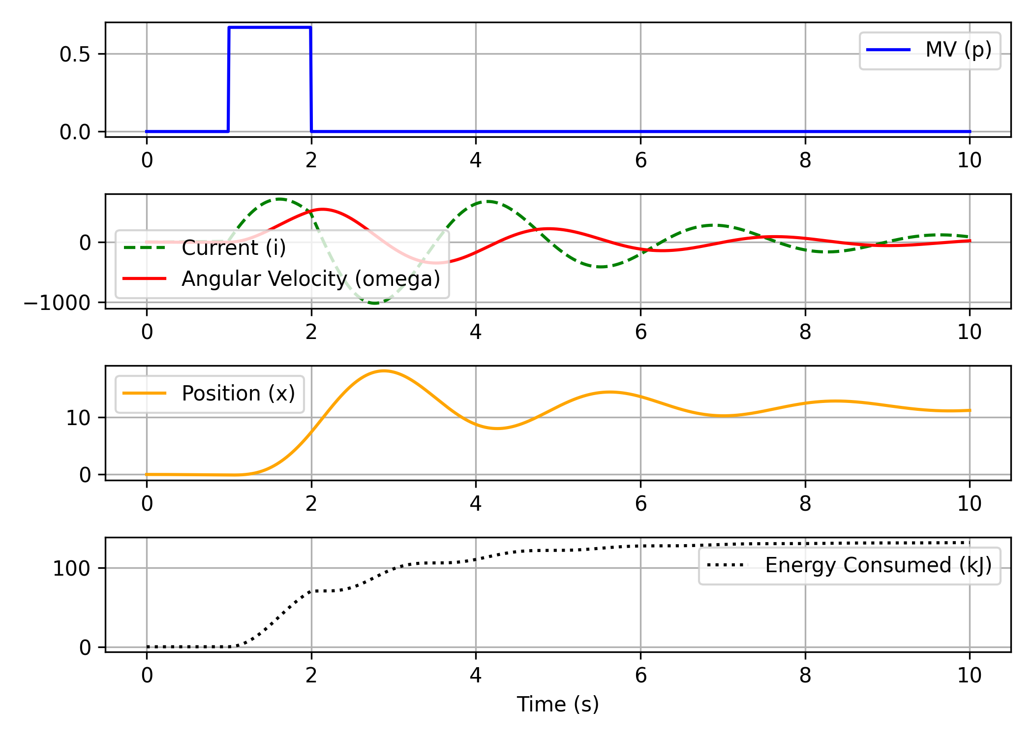
The initial simulation is a pulse in the voltage:
- `w = 0` from 0-1 sec
- `w = 100/150` from 1-1.9 sec
- `w = 0` from 1.9-10 sec
The initial simulation (non-optimal solution) is a pulse in the voltage:
- `p = 0` from 0-1 sec
- `p = 100/150` from 1-1.9 sec
- `p = 0` from 1.9-10 sec
- Manipulated variable (w) as a step input
w = m.MV(value=0) w.STATUS = 0
- Manipulated variable (p) as a step input
p = m.MV(value=0) p.STATUS = 0
w_values = np.zeros(nt) w_values[(m.time >= 1) & (m.time < 2)] = 100 / V_alim w.VALUE = w_values
p_values = np.zeros(nt) p_values[(m.time >= 1) & (m.time < 2)] = 100 / V_alim p.VALUE = p_values
i.dt() == (w * V_alim - R_m * i - K_m * omega) / L_m,
i.dt() == (p * V_alim - R_m * i - K_m * omega) / L_m,
energy.dt() == w * i * V_alim + R_bot * i**2
energy.dt() == (p * i * V_alim + R_bot * i**2)/1000
plt.plot(m.time, w.value, 'b-', label='Voltage MV (w)')
plt.plot(m.time, p.value, 'b-', label='MV (p)')
plt.plot(m.time, energy.value, 'k:', label='Energy Consumed')
plt.plot(m.time, energy.value, 'k:', label='Energy Consumed (kJ)')
Starting with this simulation model, minimize the energy to travel 100m in 10 sec. Limit the current to between -150 and +150 A to prevent damage to the battery.
The initial solution is a step-change in current with a sequence of 1-second pulses: - `i = 0` A initially - `i = 100` A for 1 second - `i = -50` A for 1 second - Back to `i = 0` A
The initial simulation is a pulse in the voltage:
- `w = 0` from 0-1 sec
- `w = 100/150` from 1-1.9 sec
- `w = 0` from 1.9-10 sec
(:title Electric Car Optimization:) (:keywords optimization, electric car, energy consumption, optimal control, nonlinear control, dynamic optimization, engineering optimization, Python, GEKKO, differential, algebraic, modeling language:) (:description Electric car optimization problem solved with Python Gekko.:)
The electric car optimization problem involves finding the optimal control strategy for driving an electric car 100 meters in 10 seconds while minimizing energy consumption. The mathematical model uses ordinary differential equations (ODEs) to describe the car behavior. The manipulated variable is the voltage input to the motor, which can accelerate or recharge the battery with regenerative braking.
The manipulated variable `w(t)` is a dimensionless variable bounded between -1 and 1. It scales the battery voltage `V_{alim}` to regulate the electric current `i(t)` in the motor:
- `w = 1` applies maximum positive voltage to accelerate the car.
- `w = -1` enables regenerative braking and recharging of the battery.
- `w = 0` disconnects the voltage supply, allowing the car to coast.
The optimal control strategy involves switching `w` strategically to minimize energy consumption while meeting constraints on position and current. This often results in a "bang-bang" control pattern, using full throttle and full braking as needed to achieve the objective efficiently.
{$ \begin{array}{llcl} \min_{e(t)} & e(T) \\ \mbox{s.t.} & \frac{di}{dt} &=& \frac{w V_{alim} - R_m i - K_m \omega}{L_m} \\ & \frac{d\omega}{dt} &=& \frac{K_r^2}{M r^2} \left( K_m i - \frac{r}{K_r} \left( M g K_f + 0.5 \rho S C_x \omega^2 \frac{r^2}{K_r^2} \right) \right) \\ & \frac{dx}{dt} &=& \frac{\omega r}{K_r} \\ & \frac{de}{dt} &=& w i V_{alim} + R_{bot} i^2 \\ & x(T) &=& 100 \\ & -150 &\leq& i(t) \leq 150 \\ & -1 &\leq& w(t) \leq 1 \end{array} $}
where `i(t)` is the electric current (A), `\omega(t)` is the angular velocity (rad/s), `x(t)` is the position of the car (m), and `e(t)` is the consumed energy (J). The manipulated variable `w(t)` regulates the current.
(:toggle hide sim button show="Electric Car Simulation":) (:div id=sim:)
The initial solution is a step-change in current with a sequence of 1-second pulses: - `i = 0` A initially - `i = 100` A for 1 second - `i = -50` A for 1 second - Back to `i = 0` A
(:source lang=python:) from gekko import GEKKO import numpy as np import matplotlib.pyplot as plt
- Create Gekko model
m = GEKKO(remote=False)
- Time discretization
nt = 1000 T = 10.0 m.time = np.linspace(0, T, nt)
- Parameters
R_bot, V_alim, R_m, K_m = 0.05, 150.0, 0.03, 0.27 L_m, r, K_r, M = 0.05, 0.33, 10.0, 250.0 g, K_f, rho, S, C_x = 9.81, 0.03, 1.293, 2.0, 0.4
- Manipulated variable (w) as a step input
w = m.MV(value=0) w.STATUS = 0
- Define the step input for current control
w_values = np.zeros(nt) w_values[(m.time >= 1) & (m.time < 2)] = 100 / V_alim w.VALUE = w_values
- Differential states
i = m.Var(value=0) omega = m.Var(value=0) x = m.Var(value=0) energy = m.Var(value=0)
- Differential equations
m.Equations([
    i.dt() == (w * V_alim - R_m * i - K_m * omega) / L_m,
    omega.dt() == (K_r**2 / (M * r**2)) * (
        K_m * i - (r / K_r) * (M * g * K_f +
        0.5 * rho * S * C_x * omega**2 * r**2 / (K_r**2))),
    x.dt() == omega * r / K_r,
    energy.dt() == w * i * V_alim + R_bot * i**2
])
- Solver options
m.options.IMODE = 4 # Simulation mode m.options.SOLVER = 3 # IPOPT solver
- Solve
m.solve(disp=True)
- Plotting the starting response
plt.figure(figsize=(7,5)) plt.subplot(4, 1, 1) plt.plot(m.time, w.value, 'b-', label='Voltage MV (w)') plt.grid(); plt.legend()
plt.subplot(4, 1, 2) plt.plot(m.time, i.value, 'g--', label='Current (i)') plt.plot(m.time, omega.value, 'r-', label='Angular Velocity (omega)') plt.grid(); plt.legend()
plt.subplot(4, 1, 3) plt.plot(m.time, x.value, color='orange', label='Position (x)') plt.grid(); plt.legend()
plt.subplot(4, 1, 4) plt.plot(m.time, energy.value, 'k:', label='Energy Consumed') plt.xlabel('Time (s)') plt.grid(); plt.legend()
plt.tight_layout() plt.savefig('sim.png',dpi=300) plt.show() (:sourceend:) (:divend:)

The Gekko Optimization Suite is a machine learning and optimization package in Python for mixed-integer and differential algebraic equations.
📄 Gekko Publication and References
The GEKKO package is available in Python with pip install gekko. There are additional example problems for equation solving, optimization, regression, dynamic simulation, model predictive control, and machine learning.