Optimize with GPR Uncertainty
Main.GPROptimization History
Hide minor edits - Show changes to markup
 GitHub |
  Google Colab GitHub | Google Colab GitHub | Google Colab GitHub | Google Colab
(:title Optimization Under Uncertainty:)
(:title Optimize with GPR Uncertainty:)

(:html:) <iframe width="560" height="315" src="https://www.youtube.com/embed/s4saLHPL14o" title="YouTube video player" frameborder="0" allow="accelerometer; autoplay; clipboard-write; encrypted-media; gyroscope; picture-in-picture" allowfullscreen></iframe> (:htmlend:)
Thanks to LaGrande Gunnell for adding the ML library to Gekko and for the example problem.
Explanation:
- Import the necessary libraries including NumPy, Matplotlib, Gekko, and Scikit-learn's Gaussian Process Regressor and kernels.
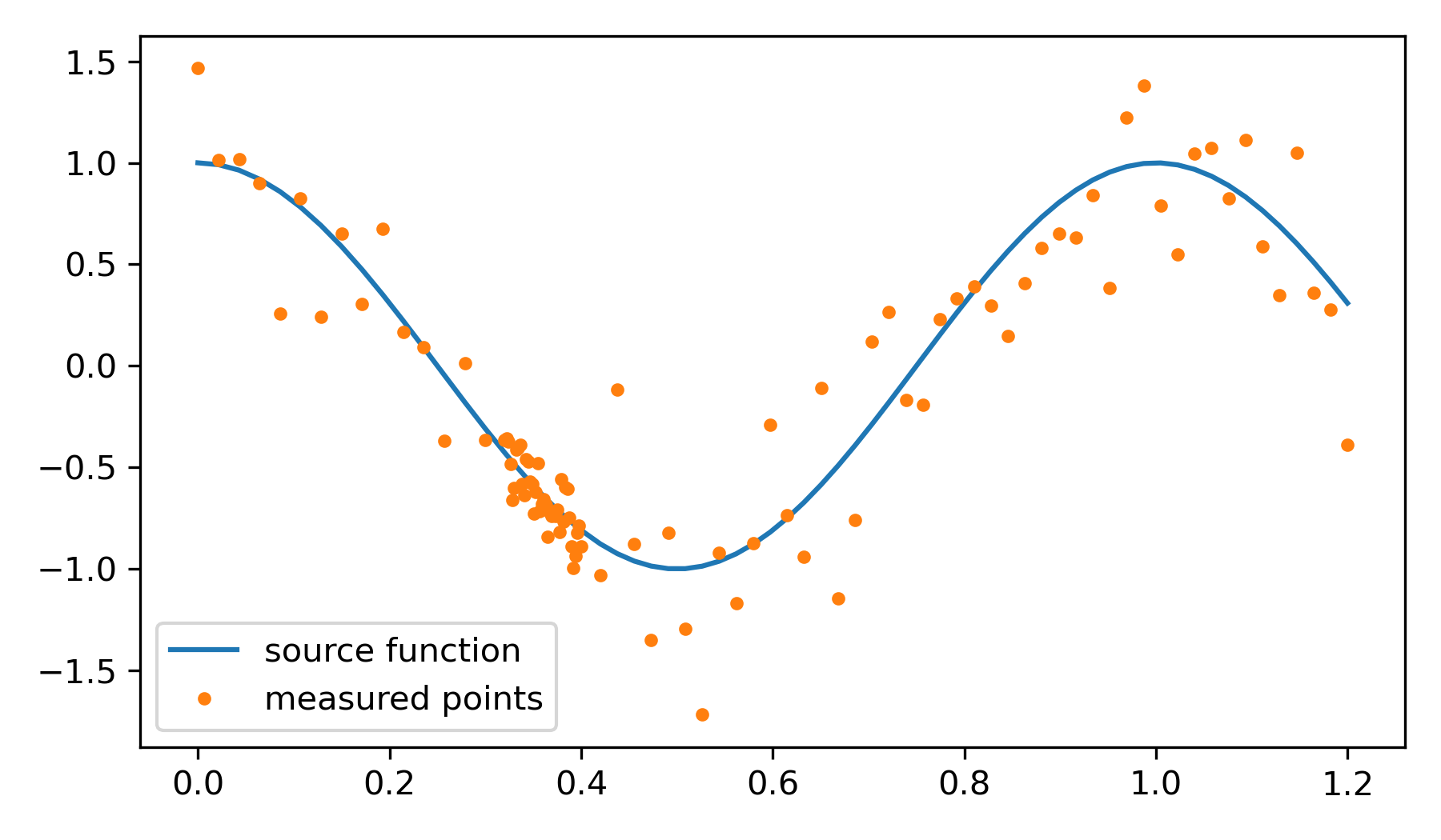
- Define the source function f(x) which includes some noise.
- Generate the data for the GPR model using the source function.
- Define the kernel and initialize the Gaussian Process Regressor.
- Fit the GPR model to the generated data.
- Set up the Gekko optimization model, define the variable and the objective function, and solve the optimization problem.
Import Libraries: Import the necessary libraries including NumPy, Matplotlib, Gekko, and Scikit-learn's Gaussian Process Regressor and kernels. Install Gekko if it isn't already installed.
from gekko import GEKKO from sklearn.gaussian_process import GaussianProcessRegressor from sklearn.gaussian_process.kernels import RBF, ConstantKernel as C
- Defining the source function
import pandas as pd import sklearn.gaussian_process as gp from sklearn.metrics import r2_score from sklearn.model_selection import train_test_split
try:
  from gekko.ML import Gekko_GPR
  from gekko import GEKKO
except:
  !pip install gekko
  from gekko.ML import Gekko_GPR
  from gekko import GEKKO
(:sourceend:)
Generate Data: Define a function to generate data with noise and visualizes this data along with the true function.
(:source lang=python:)
return np.sin(10 * x) * x + np.random.normal(0, 0.1, x.shape)
- Generating the data
np.random.seed(0) xl = np.linspace(0, 1, 100) y_true = f(xl) y_measured = f(xl)
- Define kernel and Gaussian Process Regressor
kernel = C(1.0, (1e-3, 1e3)) * RBF(0.1, (1e-2, 1e2)) gpr = GaussianProcessRegressor(kernel=kernel, n_restarts_optimizer=10)
- Fit to data
gpr.fit(xl[:, np.newaxis], y_measured)
- Optimization with Gekko
m = GEKKO(remote=False) m.x = m.Var(value=0.5, lb=0, ub=1) m.obj(f(m.x)) m.solve(disp=False)
opt_val = m.x.value
return np.cos(2*np.pi*x)
- represent noise from a data sample
N = 150 p1 = np.linspace(0.00,0.3,15) p2 = np.linspace(0.32,0.4,40) p3 = np.linspace(0.42,1.2,45) xl = np.concatenate((p1,p2,p3)) np.random.seed(14) n1 = np.random.normal(0,0.3,15) n2 = np.random.normal(0,0.1,40) n3 = np.random.normal(0,0.3,45) noise = np.concatenate((n1,n2,n3)) y_measured = f(xl) + noise
plt.figure(figsize=(6,3.5)) plt.plot(xl,f(xl),label='source function') plt.plot(xl,y_measured,'.',label='measured points') plt.legend() plt.show()
Explanation:
- Initialize another Gekko optimization model for minimizing the uncertainty.
- Define the variable and the objective function based on the GPR model's predicted standard deviation.
- Solve the optimization problem.
Data Preparation: Data is split into training and testing sets using train_test_split from scikit-learn.
- Define the Gekko optimization model for minimizing the uncertainty
m2 = GEKKO(remote=False) m2.x = m2.Var(value=0.5, lb=0, ub=1) model_pred, model_std = gpr.predict(xl[:, np.newaxis], return_std=True) m2.obj(model_std[int(m2.x.value * 100)]) m2.solve(disp=False)
opt_val2 = m2.x.value
data = pd.DataFrame(np.array([xl,y_measured]).T,columns=['x','y']) features = ['x'] label = ['y'] train,test = train_test_split(data,test_size=0.2,shuffle=True)
Explanation:
- Set up a combined optimization problem that minimizes both the GPR prediction and the uncertainty.
- Define the variable and the objective function combining both the prediction and uncertainty.
- Solve the optimization problem.
GPR Model Training: A Gaussian Process Regressor (GPR) is created and trained on the training data. The performance of the model is evaluated using the R-squared metric on the test data.
- Combined optimization for prediction and uncertainty
m3 = GEKKO(remote=False) m3.x = m3.Var(value=0.5, lb=0, ub=1) m3.Obj(f(m3.x) + model_std[int(m3.x.value * 100)]) m3.solve(disp=False)
opt_val3 = m3.x.value
k = gp.kernels.RBF() * gp.kernels.ConstantKernel() + gp.kernels.WhiteKernel() gpr = gp.GaussianProcessRegressor(kernel=k, n_restarts_optimizer=10, alpha=0.1, normalize_y=True) gpr.fit(train[features],train[label]) r2 = gpr.score(test[features],test[label]) print('gpr r2:',r2)
Explanation:
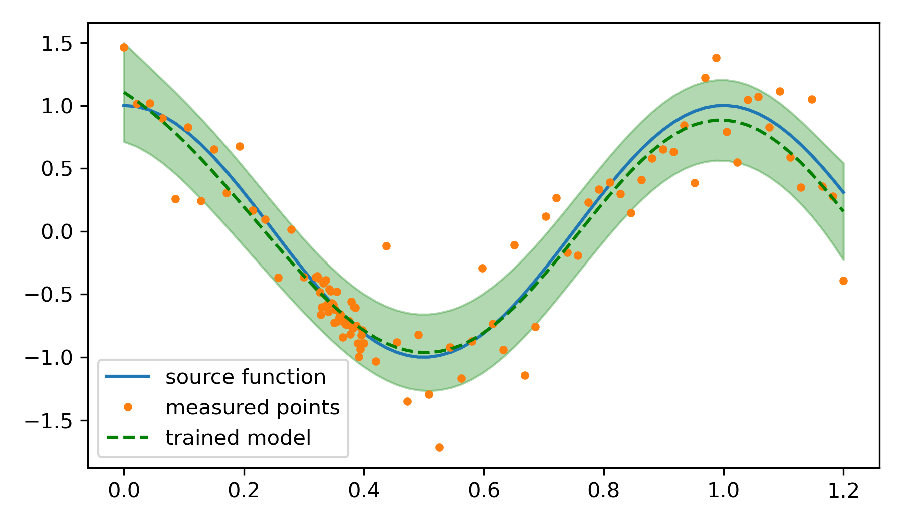
- Create a plot to visualize the source function, measured points, and GPR model.
- Add confidence intervals for the GPR model predictions.
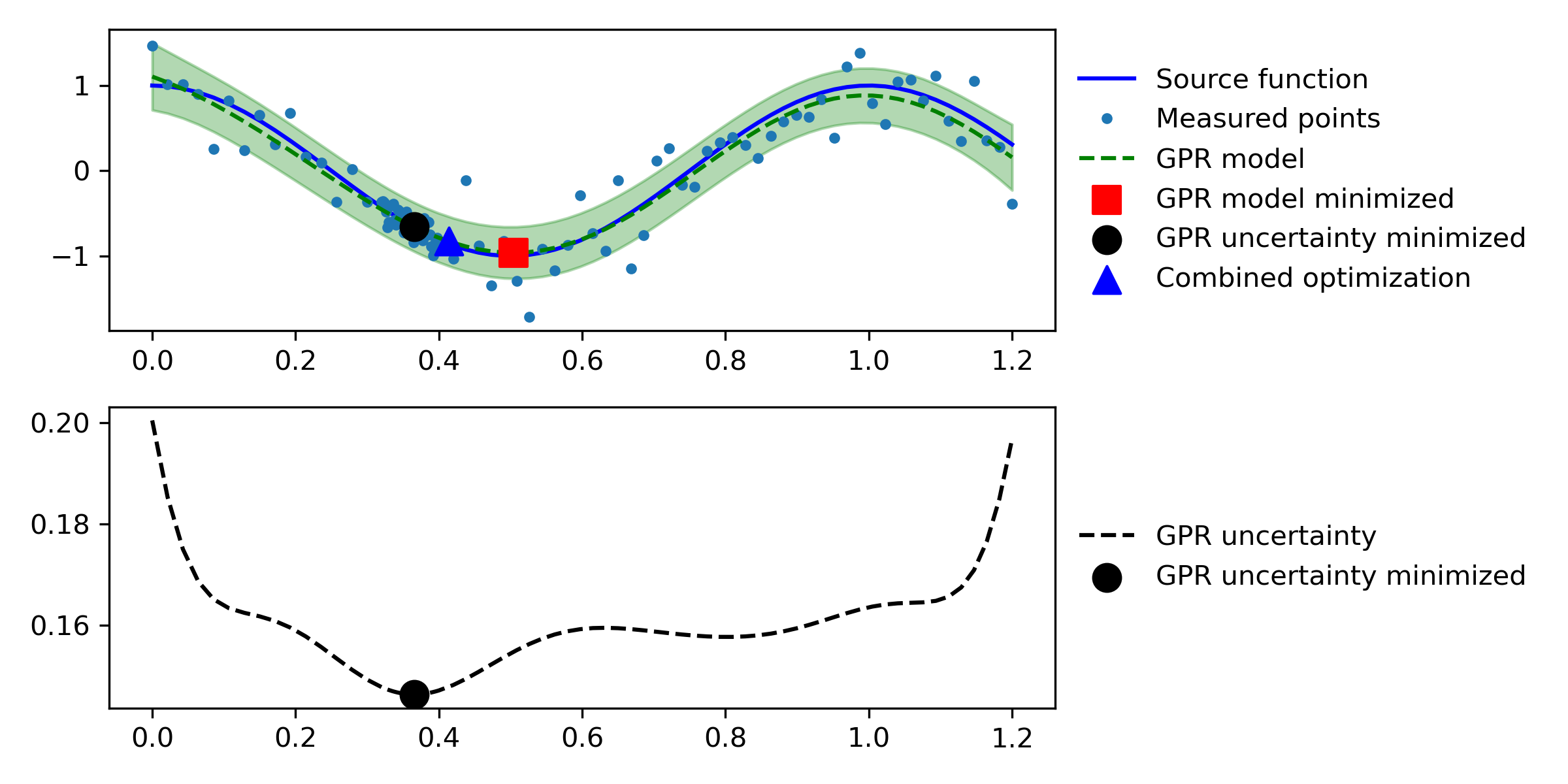
- Highlight the optimized values for the different optimization problems.
- Display the plot.
Model Visualization: The trained GPR model predictions and confidence intervals are plotted against the true function and noisy measurements.
- Plotting results
plt.figure(figsize=(8,8)) plt.subplot(2,1,1) plt.plot(xl, f(xl), 'b-', label='Source function') plt.plot(xl, y_measured, '.', label='Measured points') plt.plot(xl, model_pred, , label='GPR model', color='green') plt.fill_between(xl, model_pred - 1.96 * model_std, model_pred + 1.96 * model_std, alpha=0.3, color='green') plt.scatter([opt_val[0]], [opt_val[1]], label='GPR model minimized', color='red', marker='s', s=100, zorder=3) plt.scatter([opt_val2[0]], [opt_val2[1]], label='GPR uncertainty minimized', color='black', marker='o', s=100, zorder=3) plt.scatter([opt_val3[0]], [opt_val3[1]], label='Combined optimization', color='blue', marker='^', s=100, zorder=3) plt.legend(loc='center left', bbox_to_anchor=(1, 0.5), fontsize=10, frameon=False)
plt.subplot(2,1,2) plt.plot(xl, model_std, 'k--', label='GPR uncertainty') plt.scatter([opt_val2[0]], [opt_val2[2]], label='GPR uncertainty minimized', color='black', marker='o', s=100, zorder=3) plt.legend(loc='center left', bbox_to_anchor=(1, 0.5), fontsize=10, frameon=False)
prediction_data = pd.DataFrame(np.array([xl]).T, columns=features) model_pred, model_std = gpr.predict(prediction_data, return_std=True)
t = 1.96 #2 sided 90% Confidence interval z-infinity score
plt.plot(xl,f(xl),label='source function') plt.plot(xl,y_measured,'.',label='measured points') plt.plot(xl,model_pred,,label='trained model',color='green') plt.fill_between(xl,model_pred-t*model_std,model_pred+t*model_std,alpha=0.3,color='green') plt.legend()
Optimization with Gekko: The Gekko package is used to perform optimization. A variable is created within Gekko and the trained GPR model is used to predict the output and its uncertainty for this variable. Gekko then optimizes this variable to minimize the objective, which in this case is either the predicted value or the uncertainty of the prediction.
(:source lang=python:) m = GEKKO(remote=False) x = m.Var(0,lb=0,ub=1) y,y_std = Gekko_GPR(gpr,m).predict(x,return_std=True) m.Minimize(y) m.solve(disp=False) print('solution:',y.value[0],'std:',y_std.value[0]) print('x:',x.value[0]) print('Gekko Solvetime:',m.options.SOLVETIME,'s')
opt_val = [x.value[0],y.value[0]] (:sourceend:)
Uncertainty Optimization: uncertainty is minimized.
(:source lang=python:) m = GEKKO(remote=False) x = m.Var(0,lb=0,ub=1) y,y_std = Gekko_GPR(gpr,m).predict(x,return_std=True) m.Minimize(y_std) m.solve(disp=False) print('solution:',y.value[0],'std:',y_std.value[0]) print('x:',x.value[0]) print('Gekko Solvetime:',m.options.SOLVETIME,'s')
opt_val2 = [x.value[0],y.value[0],y_std.value[0]] (:sourceend:)
Multi-Objective Uncertainty Optimization: uncertainty and expected values are minimized as a weighted sum.
(:source lang=python:) m = GEKKO(remote=False) x = m.Var(0,lb=0,ub=1) y,y_std = Gekko_GPR(gpr,m).predict(x,return_std=True) m.Minimize(y+50*y_std) m.solve(disp=False) print('solution:',y.value[0],'std:',y_std.value[0]) print('x:',x.value[0]) print('Gekko Solvetime:',m.options.SOLVETIME,'s')
opt_val3 = [x.value[0],y.value[0],y_std.value[0]] (:sourceend:)
Results Visualization: Finally, the optimization results are visualized, showing the points of optimized predicted values and uncertainties.
(:source lang=python:) model_pred, model_std = gpr.predict(prediction_data, return_std=True)
t = 1.96 #2 sided 90% Confidence interval z-infinity score plt.figure(figsize=(8,4)) plt.subplot(2,1,1) plt.plot(xl,f(xl),'b-',label='Source function') plt.plot(xl,y_measured,'.',label='Measured points') plt.plot(xl,model_pred,,label='GPR model',color='green') plt.fill_between(xl,model_pred-t*model_std,model_pred+t*model_std,alpha=0.3,color='green') plt.scatter([opt_val[0]],[opt_val[1]],label='GPR model minimized',color='red',marker='s',s=100,zorder=3) plt.scatter([opt_val2[0]],[opt_val2[1]],label='GPR uncertainty minimized',color='black',marker='o',s=100,zorder=3) plt.scatter([opt_val3[0]],[opt_val3[1]],label='Combined optimization',color='blue',marker='^',s=100,zorder=3) plt.legend(loc='center left',bbox_to_anchor=(1, 0.5),fontsize=10,frameon=False) plt.subplot(2,1,2) plt.plot(xl,model_std,'k--',label='GPR uncertainty') plt.scatter([opt_val2[0]],[opt_val2[2]],label='GPR uncertainty minimized',color='black',marker='o',s=100,zorder=3) plt.legend(loc='center left',bbox_to_anchor=(1, 0.5),fontsize=10,frameon=False) plt.tight_layout() plt.show() (:sourceend:)
Gekko Optimization of GPR Model
Optimization Under Uncertainty
Explanation:
- Import the necessary libraries including NumPy, Matplotlib, Gekko, and Scikit-learn's Gaussian Process Regressor and kernels.
- Define the source function f(x) which includes some noise.
- Generate the data for the GPR model using the source function.
- Define the kernel and initialize the Gaussian Process Regressor.
- Fit the GPR model to the generated data.
- Set up the Gekko optimization model, define the variable and the objective function, and solve the optimization problem.
1. Import the necessary libraries including NumPy, Matplotlib, Gekko, and Scikit-learn's Gaussian Process Regressor and kernels. 2. Define the source function f(x) which includes some noise. 3. Generate the data for the GPR model using the source function. 4. Define the kernel and initialize the Gaussian Process Regressor. 5. Fit the GPR model to the generated data. 6. Set up the Gekko optimization model, define the variable and the objective function, and solve the optimization problem.
- Initialize another Gekko optimization model for minimizing the uncertainty.
- Define the variable and the objective function based on the GPR model's predicted standard deviation.
- Solve the optimization problem.
1. Initialize another Gekko optimization model for minimizing the uncertainty. 2. Define the variable and the objective function based on the GPR model's predicted standard deviation. 3. Solve the optimization problem.
- Set up a combined optimization problem that minimizes both the GPR prediction and the uncertainty.
- Define the variable and the objective function combining both the prediction and uncertainty.
- Solve the optimization problem.
1. Set up a combined optimization problem that minimizes both the GPR prediction and the uncertainty. 2. Define the variable and the objective function combining both the prediction and uncertainty. 3. Solve the optimization problem.
- Create a plot to visualize the source function, measured points, and GPR model.
- Add confidence intervals for the GPR model predictions.
- Highlight the optimized values for the different optimization problems.
- Display the plot.
plt.tight_layout() plt.savefig('combined.png', dpi=300)
Explanation: 1. Create a plot to visualize the source function, measured points, and GPR model. 2. Add confidence intervals for the GPR model predictions. 3. Highlight the optimized values for the different optimization problems. 4. Display the plot.
(:title Optimization Under Uncertainty:) (:keywords gpr, optimization, gekko, engineering, course:) (:description Optimization of Gaussian Process Regression Model using Gekko:)
Gaussian Process Regression (GPR) is a probabilistic model and non-parametric method that assumes the function is drawn from a Gaussian process. This allows the model to make predictions with well-defined uncertainty, useful for tasks such as uncertainty-aware decision-making. A more complete mathematical description is provided in the Machine Learning for Engineers course on the Gaussian Process Regression learning page.
Gekko Optimization of GPR Model
The following sections contain the code blocks for Gekko Optimization of a GPR model that minimizes the GPR prediction and uncertainty.
(:source lang=python:) import numpy as np import matplotlib.pyplot as plt from gekko import GEKKO from sklearn.gaussian_process import GaussianProcessRegressor from sklearn.gaussian_process.kernels import RBF, ConstantKernel as C
- Defining the source function
def f(x):
return np.sin(10 * x) * x + np.random.normal(0, 0.1, x.shape)
- Generating the data
np.random.seed(0) xl = np.linspace(0, 1, 100) y_true = f(xl) y_measured = f(xl)
- Define kernel and Gaussian Process Regressor
kernel = C(1.0, (1e-3, 1e3)) * RBF(0.1, (1e-2, 1e2)) gpr = GaussianProcessRegressor(kernel=kernel, n_restarts_optimizer=10)
- Fit to data
gpr.fit(xl[:, np.newaxis], y_measured)
- Optimization with Gekko
m = GEKKO(remote=False) m.x = m.Var(value=0.5, lb=0, ub=1) m.obj(f(m.x)) m.solve(disp=False)
opt_val = m.x.value (:sourceend:)
Explanation: 1. Import the necessary libraries including NumPy, Matplotlib, Gekko, and Scikit-learn's Gaussian Process Regressor and kernels. 2. Define the source function f(x) which includes some noise. 3. Generate the data for the GPR model using the source function. 4. Define the kernel and initialize the Gaussian Process Regressor. 5. Fit the GPR model to the generated data. 6. Set up the Gekko optimization model, define the variable and the objective function, and solve the optimization problem.
(:source lang=python:)
- Define the Gekko optimization model for minimizing the uncertainty
m2 = GEKKO(remote=False) m2.x = m2.Var(value=0.5, lb=0, ub=1) model_pred, model_std = gpr.predict(xl[:, np.newaxis], return_std=True) m2.obj(model_std[int(m2.x.value * 100)]) m2.solve(disp=False)
opt_val2 = m2.x.value (:sourceend:)
Explanation: 1. Initialize another Gekko optimization model for minimizing the uncertainty. 2. Define the variable and the objective function based on the GPR model's predicted standard deviation. 3. Solve the optimization problem.
(:source lang=python:)
- Combined optimization for prediction and uncertainty
m3 = GEKKO(remote=False) m3.x = m3.Var(value=0.5, lb=0, ub=1) m3.Obj(f(m3.x) + model_std[int(m3.x.value * 100)]) m3.solve(disp=False)
opt_val3 = m3.x.value (:sourceend:)
Explanation: 1. Set up a combined optimization problem that minimizes both the GPR prediction and the uncertainty. 2. Define the variable and the objective function combining both the prediction and uncertainty. 3. Solve the optimization problem.
(:source lang=python:)
- Plotting results
plt.figure(figsize=(8,8)) plt.subplot(2,1,1) plt.plot(xl, f(xl), 'b-', label='Source function') plt.plot(xl, y_measured, '.', label='Measured points') plt.plot(xl, model_pred, , label='GPR model', color='green') plt.fill_between(xl, model_pred - 1.96 * model_std, model_pred + 1.96 * model_std, alpha=0.3, color='green') plt.scatter([opt_val[0]], [opt_val[1]], label='GPR model minimized', color='red', marker='s', s=100, zorder=3) plt.scatter([opt_val2[0]], [opt_val2[1]], label='GPR uncertainty minimized', color='black', marker='o', s=100, zorder=3) plt.scatter([opt_val3[0]], [opt_val3[1]], label='Combined optimization', color='blue', marker='^', s=100, zorder=3) plt.legend(loc='center left', bbox_to_anchor=(1, 0.5), fontsize=10, frameon=False)
plt.subplot(2,1,2) plt.plot(xl, model_std, 'k--', label='GPR uncertainty') plt.scatter([opt_val2[0]], [opt_val2[2]], label='GPR uncertainty minimized', color='black', marker='o', s=100, zorder=3) plt.legend(loc='center left', bbox_to_anchor=(1, 0.5), fontsize=10, frameon=False) plt.tight_layout() plt.savefig('combined.png', dpi=300) plt.show() (:sourceend:)
Explanation: 1. Create a plot to visualize the source function, measured points, and GPR model. 2. Add confidence intervals for the GPR model predictions. 3. Highlight the optimized values for the different optimization problems. 4. Display the plot.
