Two Bar Truss Design
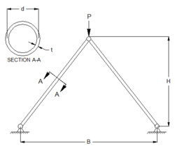
A two-bar truss is a type of truss structure consisting of two bars connected at the ends by either pins or joints. This type of truss is commonly used in construction and engineering applications.
A design of the truss is specified by a unique set of values for the analysis variables: height (H), diameter, (d), thickness (t), separation distance (B), modulus of elasticity (E), and material density (rho). Suppose we are interested in designing a truss that has a minimum weight, will not yield, will not buckle, and does not deflect "excessively,” and so we decide our model should calculate weight, stress, buckling stress and deflection.
This introductory assignment is designed as a means of demonstrating the optimization capabilities of a number of software packages. Below are tutorials for solving this problem with a number of software tools. Below are a few step-by-step tutorials.
- Two Bar APM MATLAB Tutorial
- Two Bar APM Python Tutorial
- Two Bar FMINCON MATLAB Tutorial
- Two Bar Isight Tutorial
- Two Bar Mathematica Tutorial
- Two Bar OptdesX Tutorial
Python (GEKKO) Solution
GEKKO is optimization software for mixed-integer and differential algebraic equations. It is coupled with large-scale solvers for linear, quadratic, nonlinear, and mixed integer programming (LP, QP, NLP, MILP, MINLP).

# import gekko, pip install if needed
from gekko import GEKKO
# create new model
m = GEKKO()
# declare model parameters
width = m.Param(value=60)
thickness = m.Param(value=0.15)
density = m.Param(value=0.3)
modulus = m.Param(value=30000)
load = m.Param(value=66)
# declare variables and initial guesses
height = m.Var(value=30.00,lb=10.0,ub=50.0)
diameter = m.Var(value=3.00,lb=1.0,ub=4.0)
weight = m.Var()
# intermediate variables with explicit equations
leng = m.Intermediate(m.sqrt((width/2)**2 + height**2))
area = m.Intermediate(np.pi * diameter * thickness)
iovera = m.Intermediate((diameter**2 + thickness**2)/8)
stress = m.Intermediate(load * leng / (2*area*height))
buckling = m.Intermediate(np.pi**2 * modulus \
* iovera / (leng**2))
deflection = m.Intermediate(load * leng**3 \
/ (2 * modulus * area * height**2))
# implicit equations
m.Equation(weight==2*density*area*leng)
m.Equation(weight < 24)
m.Equation(stress < 100)
m.Equation(stress < buckling)
m.Equation(deflection < 0.25)
# minimize weight
m.Minimize(weight)
# solve optimization
m.solve() # remote=False for local solve
print ('')
print ('--- Results of the Optimization Problem ---')
print ('Height: ' + str(height.value))
print ('Diameter: ' + str(diameter.value))
print ('Weight: ' + str(weight.value))
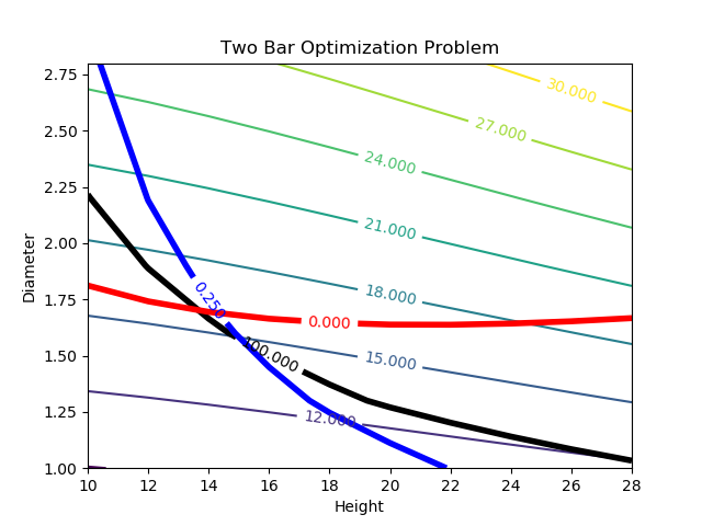
Solution Contour Plot (Python)
# Import some other libraries that we'll need
# matplotlib and numpy packages must also be installed
import matplotlib
import numpy as np
import matplotlib.pyplot as plt
# Constants
pi = 3.14159
dens = 0.3
modu = 30000.0
load = 66.0
# Analysis variables
wdth = 60.0
thik = 0.15
# Design variables at mesh points
x = np.arange(10.0, 30.0, 2.0)
y = np.arange(1.0, 3.0, 0.3)
hght, diam = np.meshgrid(x, y)
# Equations and Constraints
leng = ((wdth/2.0)**2.0 + hght**2)**0.5
area = pi * diam * thik
iovera = (diam**2.0 + thik**2.0)/8.0
wght = 2.0 * dens * leng * area
strs = load * leng / (2.0 * area * hght)
buck = pi**2.0 * modu * iovera / (leng**2.0)
defl = load * leng**3.0 / (2.0*modu * area * hght**2.0)
# Create a contour plot
# Visit https://matplotlib.org/examples/pylab_examples/contour_demo.html
# for more examples and options for contour plots
plt.figure()
# Weight contours
CS = plt.contour(hght, diam, wght)
plt.clabel(CS, inline=1, fontsize=10)
# Stress<100
CS = plt.contour(hght, diam, strs,[100.0],colors='k',linewidths=[4.0])
plt.clabel(CS, inline=1, fontsize=10)
# Deflection<0.25
CS = plt.contour(hght, diam, defl,[0.25],colors='b',linewidths=[4.0])
plt.clabel(CS, inline=1, fontsize=10)
# Stress-Buckling<0
CS = plt.contour(hght, diam, strs-buck,[0.0],colors='r',linewidths=[4.0])
plt.clabel(CS, inline=1, fontsize=10)
# Add some labels
plt.title('Two Bar Optimization Problem')
plt.xlabel('Height')
plt.ylabel('Diameter')
# Save the figure as a PNG
plt.savefig('contour1.png')
# Create a new figure to see more detail
plt.figure()
# Weight contours
CS = plt.contour(hght, diam, wght)
plt.clabel(CS, inline=1, fontsize=10)
# Stress<100
CS = plt.contour(hght, diam, strs,[90.0,100.0],colors='k',linewidths=[0.5, 4.0])
plt.clabel(CS, inline=1, fontsize=10)
# Deflection<0.25
CS = plt.contour(hght, diam, defl,[0.22,0.25],colors='b',linewidths=[0.5, 4.0])
plt.clabel(CS, inline=1, fontsize=10)
# Stress-Buckling<0
CS = plt.contour(hght, diam, strs-buck,[-5.0,0.0],colors='r',linewidths=[0.5, 4.0])
plt.clabel(CS, inline=1, fontsize=10)
# Add some labels
plt.title('Two Bar Optimization Problem')
plt.xlabel('Height')
plt.ylabel('Diameter')
# Save the figure as a PNG
plt.savefig('contour2.png')
# Show the plots
plt.show()
APM Python Tutorial
APM MATLAB Tutorial
Objective Function Plot
One part of the assignment asks you to select width and load as variables for a 3d optimal surface plot and plot the solution of the optimization problem to minimize deflection at each of the width / load combinations. This tutorial example shows how to do this same activity but for the alternative problem of minimizing weight.
 This assignment can be completed in collaboration with others. Additional guidelines on individual, collaborative, and group assignments are provided under the Expectations link.